


 texto en
  Inglés (pdf)
 Artículo en XML
 Referencias del artículo
 Enviar artículo por email
 Citado por SciELO
  Similares en
SciELO
Similares en
SciELO 
 Permalink
Introduction
Nowadays, intensive forest management practices and greater diversity of use of wood require functions for estimating trade and residual volumes of the stem with high consistency and versatility (Quiñonez, de los Santos, Álvarez, & Velázquez, 2014), supporting forest-management decision making (Rachid, Mason, Woollons, & Resquin, 2014). In this scenario, taper models continue to be an indispensable and useful tool, not only for volume point estimate, but also in the processes of simulation to optimize sawlog (Honorato, 2011; Santiago et al., 2014).
The rate of decrease in the diameter of the stem varies as we move into the height of the tree (Hjelm, 2013). The stem throughout its longitudinal extension takes different shapes depending on the species, from an neiloide in the basal region, cylindrical shapes or truncated paraboloids in the area of greatest commercial exploitation and ending in conical or parabolic shapes at the upper end of the tree (Newnham, 1992; Tamarit et al., 2014). Therefore, the greatest difficulty arises in obtaining reliable estimates of the diameter at the basal area of the stem and the apical region. In addition to the species, the profile of the stem could be determined by site productivity (Mead, 2013), sociological position of the tree in the stand and by silvicultural management activities (Matovic, Koprivica, & Radonja, 2007).
Many authors have tried to represent the profile of the stem using different mathematical models, based either on biological facts or empirical basis. The current literature includes linear taper models (Allen, 1991; Bruce et al., 1968; Kozak, Munro & Smith, 1969; Lowell, 1986; Real & Moore, 1986; Renteria & Ramirez, 1998), no linear models (Demaerschalk, 1972, 1973; Sharma & Oderwald, 2001; Sharma & Zhang, 2004), segmented models (Cao, Burkhart, & Max, 1980; Max & Burkhart, 1976; Parresol, Hotvedt, & Cao, 1987; Valenti & Cao, 1986) and trigonometric models (Thomas & Parresol, 1991). This range includes everything from differential and integral models to models that require numerical integration for obtaining stem volume.
The variety of models available today is evidence of deficiencies in the proposed models and shows stem profile model as a challenge that is still current (Gomat et al., 2011). The most common deficiencies in models relate to incorrect estimates, especially at the ends of the stem. An additional deficiency of existing models, except for a few models, is not to incorporate stand state variables that allow their widespread use, so they are valid only for the subject area of sampling and validation.
According to the above, a taper model should have the following attributes: i) be discernible along the entire length of the stem, ii) should not generate oscillations around the line of central tendency, iii) it should properly estimate not only the commercial section the stem, but also the diameter of the stump to predict the diameter at breast height and volume of the tree to rebuild the stand state variables in a post-harvest stage (Diéguez, Barrio, Castedo, & Balboa, 2003; Martínez & Acosta, 2014; Parresol, 1998) and stem volume above the limit of commercial use for sawlog and, iv) it should incorporate stand state variables to allow widespread use of the taper function arising from the model fit. Thus, the aim of this article is to fit a general nonlinear model, which requires numerical integration to obtain the respective volume function, satisfying the above criteria.
Materials and methods
Study area
The study was conducted in the central macro climatic region of Chile, which has an annual rainfall ranging between 654 and 1,949 mm (Centro de Ciencia del Clima y la Resiliencia [CR2], 2015), with a summer period of three to seven months depending on the location (Schlatter & Gerding, 1995). The tree sample was collected in stands of Pinus radiata D. Don, located in 11 municipalities in the regions of Biobío and Araucanía, in three types of soils, i.e., volcanic sand, volcanic ash and marine sediments.
Volcanic sand (VS) soils have alluvial origin and come from andesitic and basaltic volcanic sand. This type of soil is locally known as Series Arenales. These are newly formed, poorly developed soils; with thick texture in the profile and moderately thick on the surface. They form what is called the alluvial fan of the Laja, whose topography is flat with excessive drainage and rapid to very rapid permeability, although the surface runoff is slow. From late autumn to mid-spring these soils have a temporary groundwater level at depths ranging from 70 to 120 cm, which disappears in the dry season. These soils have mild to moderate wind erosion. The stands sampled in this type of soils are located in the communes of Yumbel and Cabrero.
Volcanic ash (VA) soils were formed from recent volcanic ash deposited on glaciofluvial substrates or fluvial materials, hardly detectable by the depth in which they find themselves. Poorly developed soils, deep to very deep, well-drained, with medium loam texture or silt loam superficially and silt loam in the profile, good structure, with porosity without gravels the first 160 cm, moderate permeability and moderate runoff on slopes up to 3 %. They belong to the soils known locally as Santa Bárbara with topography of low ridges and hills, with less frequent occurrence of slightly undulating soils with 2-5 % slope. The stands sampled in this type of soils are located in the communes of Coihueco, Collipulli, El Carmen, Mulchén and Quilleco. Marine sediment (MS) soils are characterized by clay loam and clay texture in the profile. They are deep reddish brown soils on the surface, well-structured soils that facilitate root development and storage of rainwater. Locally they belong to the Asociación Merilupo, which has high marine terraces topography (dissected and undulated), with moderate to strong slopes. The stands sampled in these type of soils are located in the communes of Arauco, Curanilahue, Lebu and Los Álamos.
Sample selection of stands
The study considered a total of 27 properties: nine in volcanic sand, eight in volcanic ash and 10 in marine sediments. From each property, a pine stand at harvest age was selected from cluster analysis generated based on the number of trees per hectare (N) in contrast to the basal area (G), stand state variables obtained from historical data of post-harvest inventories provided by companies participating in the study (Forestal MININCO S.A., MASISA S.A. and Forestal ARAUCO S.A.). Conglomerates were generated by the hierarchical method of Ward (Hennig, 2003, Lozada, 2010), which represent different site productivities and management intensities. A stand intended for harvest was selected from each of the most representative cluster. A sample of 10 trees in each stand was collected, covering the entire diametric spectrum recorded in the pre-harvest inventories. Overall, eliminating some trees that had errors in their records (Table 1), the sample was composed of 264 trees.
Table 1 Statistics of forest stands and trees sampled by type of soil.
| Soil / Property | N (tree·ha-1) |
G (m2 ·ha-1) |
Diameter at breast height (cm) | Total height (m) | Number of samples | |||||||
|---|---|---|---|---|---|---|---|---|---|---|---|---|
| Average | S | Min. | Max. | Average | S | Min. | Max. | Fitting | Validate | |||
| Volcanic sand | ||||||||||||
| La Aguada | 285 | 32 | 32.56 | 9.80 | 14.06 | 45.46 | 25.19 | 3.72 | 16.74 | 29.30 | 103 | 26 |
| Colicheu 8802 | 351 | 35 | 35.16 | 6.50 | 25.28 | 42.71 | 31.03 | 1.78 | 27.93 | 33.54 | 123 | 30 |
| Cerro Verde 8618 | 1,288 | 43 | 23.53 | 10.99 | 9.56 | 39.32 | 21.58 | 5.42 | 11.72 | 28.08 | 94 | 24 |
| Colicheu 9132 | 1,190 | 35 | 21.09 | 7.09 | 10.05 | 31.47 | 20.13 | 4.73 | 12.00 | 26.72 | 87 | 21 |
| Tapihue | 491 | 32 | 26.62 | 8.60 | 14.69 | 39.15 | 27.63 | 4.54 | 19.62 | 34.44 | 106 | 28 |
| Cerro Verde 8605 | 1,022 | 48 | 27.40 | 9.45 | 11.00 | 41.74 | 27.43 | 4.44 | 17.94 | 31.60 | 109 | 28 |
| El Membrillo | 1,201 | 25 | 18.52 | 6.25 | 10.69 | 28.00 | 17.38 | 3.08 | 12.76 | 21.58 | 77 | 19 |
| San Cristóbal 9403 | 1,620 | 51 | 25.67 | 11.11 | 8.04 | 40.00 | 23.74 | 5.00 | 13.65 | 29.07 | 100 | 27 |
| San Cristóbal 9801 | 751 | 59 | 30.65 | 8.71 | 18.10 | 43.30 | 28.44 | 3.12 | 22.57 | 32.60 | 114 | 31 |
| Subtotal | 913 | 234 | ||||||||||
| Volcanic ash | ||||||||||||
| El Mogoto Hijuela 2 | 369 | 47 | 37.97 | 14.77 | 13.59 | 58.64 | 31.60 | 7.27 | 17.42 | 39.10 | 104 | 36 |
| Las Malvinas | 590 | 53 | 33.12 | 9.86 | 19.02 | 46.87 | 30.43 | 6.08 | 21.03 | 38.31 | 116 | 33 |
| Santa Julia | 512 | 46 | 33.09 | 7.76 | 21.51 | 44.78 | 29.13 | 4.15 | 18.94 | 32.60 | 110 | 31 |
| Santa Edelmira | 352 | 43 | 36.69 | 7.68 | 24.34 | 49.49 | 34.86 | 3.51 | 29.20 | 39.72 | 137 | 30 |
| Coleal | 500 | 43 | 33.55 | 11.28 | 14.65 | 48.37 | 30.74 | 4.88 | 20.94 | 37.33 | 125 | 35 |
| Parc Collipulli | 396 | 43 | 36.97 | 11.26 | 22.29 | 54.44 | 32.41 | 3.60 | 25.90 | 37.41 | 121 | 32 |
| Nahueltoro | 410 | 49 | 35.04 | 10.92 | 17.17 | 49.23 | 30.21 | 4.74 | 20.20 | 34.00 | 71 | 13 |
| Los Molinos | 295 | 42 | 35.63 | 14.77 | 15.72 | 57.70 | 30.54 | 5.77 | 22.14 | 37.05 | 119 | 32 |
| Subtotal | 903 | 242 | ||||||||||
| Marine sediments | ||||||||||||
| Quemas II | 346 | 51 | 42.71 | 8.24 | 29.98 | 55.00 | 39.19 | 2.78 | 33.78 | 44.83 | 150 | 38 |
| La Colcha | 338 | 46 | 36.56 | 12.57 | 15.65 | 56.68 | 32.20 | 5.04 | 21.37 | 37.92 | 127 | 31 |
| Ranquil La Loma | 364 | 63 | 42.62 | 9.79 | 27.56 | 59.93 | 32.83 | 3.06 | 26.63 | 35.60 | 85 | 29 |
| El Rosal 2 | 740 | 74 | 30.31 | 13.41 | 9.64 | 49.50 | 30.12 | 9.27 | 16.65 | 41.80 | 111 | 22 |
| La Araucana | 1,467 | 82 | 34.60 | 11.03 | 14.10 | 48.99 | 31.96 | 5.03 | 20.82 | 36.47 | 122 | 32 |
| La Araucana | 642 | 58 | 31.61 | 10.08 | 13.44 | 44.96 | 34.14 | 8.29 | 18.04 | 46.00 | 123 | 26 |
| El Blanco | 960 | 74 | 35.20 | 11.51 | 12.03 | 50.58 | 31.68 | 6.35 | 15.84 | 36.10 | 118 | 28 |
| Chupalla | 435 | 49 | 37.69 | 9.41 | 26.86 | 58.72 | 32.48 | 2.36 | 26.93 | 36.17 | 118 | 30 |
| Peumo Sur | 352 | 47 | 39.24 | 8.50 | 25.20 | 49.98 | 34.50 | 3.64 | 27.26 | 39.00 | 124 | 31 |
| Chicaucura | 475 | 55 | 42.56 | 14.75 | 16.68 | 63.94 | 33.94 | 6.93 | 19.13 | 40.00 | 112 | 30 |
| Subtotal | 1190 | 297 | ||||||||||
N: planting density; G: basal area; S: standard deviation; Min.: minimum; Max.: maximum.
Destructive sampling of trees
At 1.30 m of each standing tree the diameter at breast height (DBH) was measured and marked. Once the tree was felled, we measured the total height and the stem was marked every 2 m from the dbh up to reaching the limit diameter of utilization (ldu) of 8 cm. From there on, the stem was marked every 1 m. Then a slice from the base of the tree (stump) was extracted, another at dbh and then every 2.44 m until reaching the height of ldu to facilitate the commercial use of the resulting logs. Slices were extracted every 1 m, from the ldu, up to a diameter not less than 2.54 cm. In the laboratory, the average diameter without bark was determined for each slice and, from this we estimate the volume without bark of each stem section between each pair of successive slices, using the formula of Smalian:

where:
V = |
volume without bark of each stem section (m3) |
L = |
length of the section (m) |
Au = |
upper area of each section (m2) |
Al = |
lower area of each section (m2) |
The total volume of each tree was determined from the sum of the volumes of their respective sections. Measuring the diameters of the upper area of the stem above the ldu is very important for proper determination of the total volume (de Miguel, Mehtätalo, Shater, Kraid, & Pukkala, 2012).
Stem Profile Model
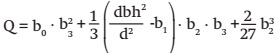
A series of preliminary tests of trial and error allowed to determine the empirical model to represent adequately the dimensions in its entirety and that would have continuity along the stem, including the basal section and the upper end, depending on measures concerning the tree and stand state variables. Tests were performed to each of the taper model parameters obtained (including modeling of multiple linear regressions using stand state variables as predictors) and the model with the smallest index of the Akaike information criterion (AIC) (Akaike, 1974) was chosen between different alternative forms, which gave form to the following generalized model:
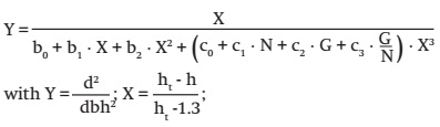 [1]
[1]
where:
d = |
diameter without bark (cm), from the slice obtained at the height h (m) |
dbh = |
diameter at breast height (cm) at 1.30 m |
ht = |
total height of the tree (m) |
N = |
density of the stand (trees·ha-1) |
G = |
basal area of the stand (m2·ha-1) |
b0, b1, b2, c0, c1, c2, c3, |
are model parameters |
However, some additional tests allow greater stability of the model in the basal region by replacing in the previous model the function that represents the stand state variables by a new parameter.
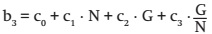 [2]
[2]
where:
N = |
Stand density (trees·ha-1) |
G = |
Basal area of the stand (m2·ha-1) |
b3, c0, c1, c2 and c3, |
are model parameters |
By implementing this parameter, the initial model proposed is not only simplified, but in turn the parameters b0, b1 and b2 are considered as constant values; based on such parameters that were adjusted in the generalized model [1], which considered in its adjustment the presence of the stand state variables. Thus, the following generalized and simplified model is obtained:
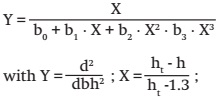 [3]
[3]
where:
d = |
diameter without bark (cm) from the slice obtained at height h (m) |
dbh = |
diameter at breast height (cm) a 1.30 m |
ht = |
Total height of the tree (m) |
b3 = |
parameter to be fitted |
b0, b1 and b2, |
are constant values obtained from the model fit [1] |
From the linear expression of the generalized and simplified model [3] and then represented algebraically in the same way that the equation of Tartaglia-Cardano (Kichenassamy, 2015), we can get any height according to their respective diameter through the following transformation of variables:
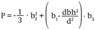 [4]
[4]
 [5]
[5]
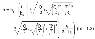 [6]
[6]
where:
h = |
height (m) in the stem of the slice of diameter d (cm) without bark |
dbh = |
diameter at breast height (cm) at 1.30 m |
ht = |
total height of the tree (m) |
b0, b1 and b2, |
are the parameters obtained from fitting the model [1] |
b3 = |
parameter obtained from fitting the model [3] |
P and Q, |
are transformations of the linear representation of the model [3], to make use of the formula of Tartaglia- Cardano. |
The comparison of the variability of the parameters of the generalized model [1] according to the type of soil was performed using the F-test, of Fisher and Snedecor, where the variation of the sum of the squared error was evaluated under the following hypothesis:
H0: The taper model does not differ among different types of soils.
H1: The taper model differs among different types of soils, in at least some of its parameters.
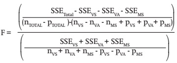
where:
SSE = |
sum of squares error |
n = |
number of samples |
p = |
number of parameters of the model |
VS: |
Volcanic sand; VA: Volcani ash; MS: Marine sediments. |
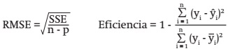
Fitting nonlinear models was performed by the method NLIN (SAS, 2009). In the case of the assessment of the accuracy of fitting the taper model, we use the root mean square error (RMSE) and an indicator of predictive model efficiency
Quantifying the volume from the taper model
The taper model was integrated numerically using the IML procedure (SAS, 2009). To quantify the volume only the generalized and simplified model [3] developed in this paper was considered. The procedure was used to estimate the volume of each tree from the database for validation from the parameters obtained in the fitting of the taper model, and was compared with the volume determined by the formula of Smalian through cross-validation between the estimated value and the observed value by a simple linear regression. Previously, 75 % of the samples were selected for fitting and, 25 % of the samples for validation. None of the samples selected for validation of model was used for model fitting, in order to assure the independence of the samples (de Miguel et al., 2012).
Comparison of taper model
To compare the fitting of the generalized and simplified model [3], in contrast to the taper model with the same response variable published in the scientific literature by other authors (Table 2), the Akaike information criterion (AIC) (Akaike, 1974), the root mean square error (RMSE) were used and the significant differences among the various models were compared through a Turkey’s multiple range test LSD (95 % confidence level) from the individual values observed when obtaining the mean absolute error (MAE).
Table 2 Linear, nonlinear, segmented and trigonometric taper models.
| Model | Authors |
|---|---|
| Bruce, Curtis, y Vancoevering (1968) | |
| Kozak, Munro, & Smith (1969) | |
| Demaerschalk (1972) | |
| Demaerschalk (1973) | |
| Coffre (Rojo et al. (2005) | |
| Lowell (1986) | |
| Real & Moore (1986) | |
| Rentería & Ramírez (1998) | |
| Sharma & Zhang (2004) | |
|
|
Max & Burkhart (1976) |
|
|
Max & Burkhart (1976) |
|
|
Cao, Burkhart & Max (1980) Modified |
|
|
Valenti & Cao (1986) |
|
|
Parrestol, Hotvedt, & Cao (1987) |
| Thomas & Parresol (1991) |
With
where:
This study does not consider the model proposed by Munro, quoted by Rojo, Perales, Sánchez, Álvarez and Von Gadow (2005), since when considering the stem profile as a straight line, underestimates the diameter both in the basal area as in the apical area. Likewise, the models of Allen (1991) and Sharma and Oderwald (2001) were excluded for analysis and comparison purposes due to its slow adjustment in the three different types of soil. Only those taper models with the highest accuracy, lowest bias, best graphic performance of the trendline, and proper random distribution of residuals versus predicted values were selected for comparative analysis.
Results and discussion
The generalized model [1] shows consistency in all the parameters (P < 0.05) in sand and volcanic ash (Table 3), except parameter c3, which is not statistically significant for marine sediments.
Table 3 Model parameters for predicting the stem profile of Pinus radiata for each type of soil in the Biobío and Araucanía regions of Chile.
| Soil | n | b0 | b1 | b2 | c0 | c1 | c2 | c3 | RMSE |
|---|---|---|---|---|---|---|---|---|---|
| VS | 913 | 4.5355* | -12.7521* | 17.5378* | -8.2431* | 0.000086* | -0.00130* | 1.3839* | 0.04919 |
| VA | 903 | 4.3156* | -12.9686* | 18.6764* | -8.4626* | -0.000950* | 0.01010* | -4.1966* | 0.05109 |
| MS | 1190 | 4.0928* | -12.5876* | 18.8387* | -9.0158* | 0.000094* | -0.00401* | n.s. | 0.05206 |
VS: Volcanic sand, VA: Volcanic ash, MS: Marine sediments. n: number of samples; b0, b1, b2, c0, c1, c2, c3: model parameters; RMSE: root mean square error; *: Significant at P<0.05; n.s.: non-significant.
In the case of the generalized and simplified model [3], we obtained high efficiency in predicting the stem profile (Table 4), whose parameters differ significantly among the different types of soil (F-test).
Table 4 Generalized model parameters for predicting the stem profile of Pinus radiata for each type of soil in the Biobío and Araucanía regions of Chile.
| Soil | n | b0 | b1 | b2 | b3 | RMSE | Efficiency (%) | F-test |
|---|---|---|---|---|---|---|---|---|
| VS | 913 | 4.5355* | -12.7521* | 17.5378* | -8.1364* | 0.04930 | 97.24 | |
| VA | 903 | 4.3156* | -12.9686* | 18.6764* | -8.8734* | 0.05263 | 97.19 | |
| MS | 1190 | 4.0928* | -12.5876* | 18.8387* | -9.1970* | 0.05128 | 96.91 | |
| Total | 3006 | 4.2923* | -12.7645* | 18.4243* | -8.7917* | 0.05244 | 93.93 | 18.15 |
VS: Volcanic sand, VA: Volcanic ash, MS: Marine sediments. n: number of samples; b0, b1, b2, b3: model parameters; RMSE: root mean square error; *: Significant at P<0.05; n.s.: non-significant.
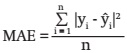
Generalized and simplified [3] model presents high flexibility in the representation of the stem profile, which allows to estimate both the basal diameters and the diameters of the upper part of the stem (Figure 1). Normally these stem sectors do not represent a commercial use for sawlog purposes. However, the flexibility of the model is important to quantify the crown biomass for energy purposes. Figure 1 shows that the curves adequately describe the behavior of the data, the entire profile of the stem.
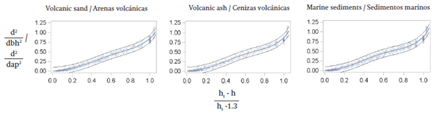
Figure 1 Taper model for Pinus radiata according to the distance to the apex regarding the diameter at breast height, with the limits of upper and lower confidence at 95 %.
For that reason parameterization adequately represent the different types of soil according to the stand state variables, whose residuals were randomly distributed around the line 0 (Figure 2) in each type of soil.
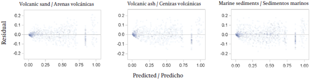
Figure 2 Residuals of the generalized and simplified model [3] in the representation of the stem profile of Pinus radiata .
The volume obtained via integration by numerical methods of the generalized and simplified taper model [3], being validated crosswise based on the sum of the volumes obtained in each log by the formula of Smalian, has a prediction efficiency above 97 % (Figure 3).
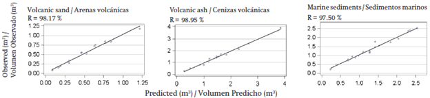
Figure 3 Validation of the volume of Pinus radiata the stem without bark, for each type of soil in the regions of Biobío and the Araucanía, Chile .
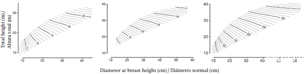
For graphical representation of the height model [6] obtained from generalized and simplified model [3], a diameter without bark of 8 cm (Figure 4) was considered, based on commercial requirements of thin tip for sawlog purposes.
Comparison of some taper models published by other authors
Most models converged in all parameters (Table 5), except the models of Coffre cited by Rojo et al. (2005) [11] and Renteria and Ramirez (1998) [14], which showed some parameter nonsignificant in each of the different types of soils, and the model of Lowell (1986) [12] in the case of volcanic sand soils. The root mean square error (RMSE) ranged between 0.04827 and 0.12124, and the mean absolute error (MAE) between 0.03485 and 0.07482 (Table 6).
Table 5 Parameters of the Pinus radiata taper models for each type of soil in the Biobío and Araucanía regions of Chile.
| Model | Method | b0 | b1 | b2 | b3 | b4 | b5 | a | a1 | a2 |
|---|---|---|---|---|---|---|---|---|---|---|
| Volcanic sand | ||||||||||
| 7 | N | 0.9585* | -0.1827* | 0.0424* | ||||||
| 8 | N | -1.4635* | 0.5385* | |||||||
| 9 | N | 0.9124* | 1.4520* | |||||||
| 10 | N | 2088.2* | 32.6328* | 0.8741* | 1.3796* | |||||
| 11 | N | 0.3584* | 0.4921* | n.s. | ||||||
| 12 | N | 0.2437* | n.s. | 5.0080* | -9.0396* | 4.6342* | ||||
| 13 | N | -2.0653* | 0.7759* | -0.0497* | ||||||
| 14 | N | 0.3866* | 0.5385* | n.s. | ||||||
| 15 | N | 0.8103* | -0.0798* | 0.2273* | -0.5307* | |||||
| 16 | N | -1.3379* | 0.4502* | 62.3298* | 0.0490* | |||||
| 17 | M | -2.3653* | 1.0777* | 24.7515* | 0.0889* | 0.6538* | ||||
| 18 | M | -1.1064* | 2.8525* | -98.4159* | 0.2018* | 0.9407* | ||||
| 19 | M | n.s. | 2.0666* | -0.8441* | -1.2086* | 0.2954* | 0.5736* | |||
| 20 | N | 2.1247* | -1.4430* | -56.1255* | 24.4860* | 0.7640* | ||||
| 21 | N | -0.7370* | 0.0544* | 0.0023* | ||||||
| Volcanic ash | ||||||||||
| 7 | N | 1.0996* | -0.3389* | 0.6960* | ||||||
| 8 | N | -1.3967* | 0.4694* | |||||||
| 9 | N | 0.9150* | 1.3774* | |||||||
| 10 | N | 9087.5* | 172.70* | 0.8791* | 1.3073* | |||||
| 11 | N | 0.4369* | 0.4329* | n.s. | ||||||
| 12 | N | 0.5098* | -2.0307* | 11.3241* | -16.8735* | 7.9383* | ||||
| 13 | N | -2.3690* | 0.8031* | -0.4340* | ||||||
| 14 | N | 0.4580* | 0.4694* | n.s. | ||||||
| 15 | N | 0.8267* | -0.0840* | 0.3023* | -0.5372* | |||||
| 16 | N | -1.2161* | 0.3418* | 106.30* | 0.0438* | |||||
| 17 | M | -2.6557* | 1.2067* | 72.6528* | 0.0574* | 0.7146* | ||||
| 18 | M | -1.3929* | 4.0970* | -249.50* | 0.2718* | 0.9437* | ||||
| 19 | M | 0.0996* | 1.9546* | -0.7954* | -1.2158* | 0.2857* | 0.5648* | |||
| 20 | N | 2.2283* | -1.5149* | -385.0* | 148.00* | 0.8672* | ||||
| 21 | N | -0.7737* | 0.0446* | 0.0013* | ||||||
| Marine sediments | ||||||||||
| 7 | N | 1.1271* | -0.3817* | 0.0819* | ||||||
| 8 | N | -1.3406* | 0.4273* | |||||||
| 9 | N | 0.9011* | 1.3426* | |||||||
| 10 | N | 11170* | 256.70* | 0.8708* | 1.2815* | |||||
| 11 | N | 0.0075* | n.s. | 0.2789* | ||||||
| 12 | N | 0.5231* | -1.8834* | 11.0539* | -17.0375* | 8.2149* | ||||
| 13 | N | -2.6282* | 0.8991* | -0.4420* | ||||||
| 14 | N | 0.3120* | n.s. | 0.3120* | ||||||
| 15 | N | 0.8257* | -0.0785* | 0.2410* | -0.4129* | |||||
| 16 | N | -1.1276* | 0.2761* | 99.9986* | 0.0476* | |||||
| 17 | M | -3.0469* | 1.4020* | 64.6872* | 0.0632* | 0.7705* | ||||
| 18 | M | -1.4286* | 4.3943* | -205.30* | 0.2505* | 0.9350* | ||||
| 19 | M | 0.0706* | 2.1677* | -1.0112* | -1.3212* | 0.2963* | 0.5656* | |||
| 20 | N | 2.3376* | -1.6851* | -213.8* | 85.5204* | 0.8333* | ||||
| 21 | N | -0.7990* | 0.0285* | 0.0002* | ||||||
M and N: Marquardt and Newton convergence method, respectively; b0, b1, b2, b3, b4, b5, a, a1, a2: model parameters; *: Significant at P < 0.05; n.s.: non-significant.
Table 6 Statistics of the Pinus radiata taper models for each type of soil in the Biobío and Araucanía regions of Chile.
| Model | Number of data | AIC | RMSE | MAE | LSD Turkey test | |||||||
|---|---|---|---|---|---|---|---|---|---|---|---|---|
| Volcanic Sand | ||||||||||||
| 3 | 913 | -5488.46 | 0.04930 | 0.03563 | a | b | ||||||
| 7 | 913 | -5513.26 | 0.04879 | 0.03525 | a | b | ||||||
| 8 | 913 | -5306.10 | 0.05468 | 0.03929 | a | b | ||||||
| 9 | 913 | -5302.05 | 0.05477 | 0.03790 | a | b | ||||||
| 10 | 913 | -5439.41 | 0.05070 | 0.03617 | a | b | ||||||
| 11 | 913 | -5309.70 | 0.05450 | 0.03902 | a | b | ||||||
| 12 | 913 | -5480.88 | 0.04960 | 0.03565 | a | b | ||||||
| 13 | 913 | -4773.25 | 0.07314 | 0.04746 | c | d | ||||||
| 14 | 913 | -5306.10 | 0.05468 | 0.03929 | a | b | ||||||
| 15 | 913 | -5479.25 | 0.04960 | 0.03592 | a | b | ||||||
| 16 | 913 | -5436.45 | 0.05079 | 0.03819 | a | b | ||||||
| 17 | 913 | -5483.09 | 0.04950 | 0.03526 | a | b | ||||||
| 18 | 913 | -5492.61 | 0.04919 | 0.03485 | a | |||||||
| 19 | 913 | -5390.46 | 0.05206 | 0.03670 | a | b | ||||||
| 20 | 913 | -5445.88 | 0.05050 | 0.03627 | a | b | ||||||
| 21 | 913 | -5127.93 | 0.06025 | 0.04183 | b | c | ||||||
| Volcanic Ash | ||||||||||||
| 3 | 903 | -5358.45 | 0.05128 | 0.03753 | a | b | c | |||||
| 7 | 903 | -5469.17 | 0.04827 | 0.03574 | a | |||||||
| 8 | 903 | -5096.02 | 0.05941 | 0.04354 | c | d | ||||||
| 9 | 903 | -5089.38 | 0.05967 | 0.04241 | a | b | c | d | ||||
| 10 | 903 | -5316.28 | 0.05254 | 0.03840 | a | b | c | |||||
| 11 | 903 | -5129.08 | 0.05840 | 0.04276 | b | c | d | |||||
| 12 | 903 | -5356.64 | 0.05138 | 0.03804 | a | b | c | |||||
| 13 | 903 | -4786.27 | 0.07050 | 0.04768 | d | e | f | |||||
| 14 | 903 | -5096.02 | 0.05941 | 0.04354 | c | d | ||||||
| 15 | 903 | -5462.62 | 0.04848 | 0.03571 | a | |||||||
| 16 | 903 | -5329.69 | 0.05215 | 0.03993 | a | b | c | |||||
| 17 | 903 | -5404.38 | 0.05000 | 0.03672 | a | b | ||||||
| 18 | 903 | -5402.54 | 0.05000 | 0.03670 | a | b | ||||||
| 19 | 903 | -5195.76 | 0.05612 | 0.04040 | a | b | c | |||||
| 20 | 903 | -5327.62 | 0.05215 | 0.03831 | a | b | c | |||||
| 21 | 903 | -4994.01 | 0.06285 | 0.04417 | c | d | e | |||||
| Marine Sediments | ||||||||||||
| 3 | 1190 | -7000.99 | 0.05263 | 0.03853 | a | |||||||
| 7 | 1190 | -7097.18 | 0.05060 | 0.03714 | a | |||||||
| 8 | 1190 | -6582.55 | 0.06285 | 0.04610 | c | d | e | f | ||||
| 9 | 1190 | -6558.22 | 0.06348 | 0.04486 | b | c | d | e | ||||
| 10 | 1190 | -6822.06 | 0.05683 | 0.04150 | a | b | c | d | ||||
| 11 | 1190 | -6646.60 | 0.06124 | 0.04657 | d | e | f | g | ||||
| 12 | 1190 | -6998.74 | 0.05273 | 0.03918 | a | b | ||||||
| 13 | 1190 | -6302.84 | 0.07071 | 0.04835 | e | f | g | h | ||||
| 14 | 1190 | -6601.24 | 0.06237 | 0.04739 | d | e | f | g | h | |||
| 15 | 1190 | -7076.32 | 0.05109 | 0.03797 | a | |||||||
| 16 | 1190 | -6961.96 | 0.05357 | 0.04185 | a | b | c | d | ||||
| 17 | 1190 | -7040.06 | 0.05177 | 0.03825 | a | |||||||
| 18 | 1190 | -7038.36 | 0.05187 | 0.03823 | a | |||||||
| 19 | 1190 | -6749.97 | 0.05848 | 0.04217 | a | b | c | d | ||||
| 20 | 1190 | -6911.61 | 0.05468 | 0.04022 | a | b | c | |||||
| 21 | 1190 | -6190.99 | 0.07409 | 0.05286 | h | |||||||
AIC: Akaike information criterion; RMSE: root mean square error; MAE: mean absolute error. Note: LSD Tukey test was performed independently for each type of soil
Graphical analysis of the residuals were determined to select models with greater stability and better performance to describe the tendency of the taper model. For example, the models of Kozak et al. (1969) [8], Demaerschalk (1972) [9], Coffre (Rojo et al., 2005) [11], Renteria and Ramirez (1998) [14], Valenti & Cao (1986) [19] and Thomas and Parresol (1991) [21], even when considering curved the stem profile, underestimating the diameter of the basal area of the stem. Additionally, the model of Thomas and Parresol (1991) [21] underestimates the stem profile at diameter at breast height.
Other models showed overestimates of the stem profile, such as the models of Demaerschalk (1972) [9] Real and Moore (1986) [13], Renteria and Ramirez (1998) [14] and Valenti and Cao (1986) [19] showing estimates of the diameter at breast height above the observed value, which overestimates the supply of timber for sawlog purposes. The models of Kozak et al. (1969) [8], Coffre (Rojo et al., 2005) [11], Renteria and Ramirez (1998) [14], Sharma and Zhang (2004) [15], Max and Burkhart (1976) [16], Cao et al. (1980) [18] y Thomas and Parresol (1991) [21] overestimated the diameter of the apical part of the stem, which leads to overestimated estimates of the biomass supply above ldu, such as biomass for energy purposes.
Similarly, models having high sensitivity, which is manifested in oscillations around the line of estimation were observed, this is common in polynomials of high degree, as presented in the graphical representation of models of Demaerschalk (1973) [ 10] and Sharma and Zhang (2004) [15]. Meanwhile, the model [19] of Valenti and Cao (1986) is continuous but not differentiable at the junction points, which increases the variability in prediction of the diameter of the stem profile, at heights near these points.
Some models showed abrupt changes below the diameter at breast height, with trend lines that have little natural breaks in the case of Pinus radiata, models of Bruce et al. (1968) [7], Demaerschalk (1973) [10], Real and Moore (1986) [13], Max and Burkhart (1976) [16] y [17], Cao et al. (1980) [18], Parresol et al. (1987) [20] and Thomas and Parresol (1991) [21].
The generalized and simplified taper model [3] did not differ significantly (LSD Tukey Test, 95 % confidence level) from those models that had the best fittings for the three types of soil (Table 6): models of Bruce et al. (1968) [7], Demaerschalk (1973) [10], Lowell (1986) [12], Sharma and Zhang (200) [15], Max and Burkhart (1976) [16] and [17] Cao et al. (1980) [18], Valenti and Cao (1986) [19] and Parresol et al. (1987) [20]. The generalized and simplified model [3] proposed in this study does not show any of the inconsistencies observed in other models.
On the other hand, the model [11] of Coffre, cited by Rojo et al. (2005), with which the Forestry Institute of Chile (INFOR) developed the compendium of auxiliary tables for managing Pinus radiata (Peters, Jobet, & Aguirre, 1985), expresses its parameters depending on the age of the plantation. However, Table 6 shows that the generalized and simplified taper model [3] has a better fit in volcanic ash soils and marine sediments, and differs significantly by the LSD Tukey Test (95 %, confidence level), with the aggravation that the model of Coffre had some non-significant parameter in all types of soils.
Conclusions
The proposed generalized and simplified taper model showed differentiation of parameters for each type of soil, i.e. volcanic sand and ash and marine sediments, according to the planting density and basal area expressed intrinsically. The variable age is not significant in obtaining the generalized model.
The statistical goodness of fit and predictive statistics of the model proposed showed its efficiency to estimate the profile and volume of the stem without bark of Pinus radiata (from base to apex) on each of the different types of soil.
By contrasting the model proposed with different taper models having the same response variable, no significant difference was observed from those models that had the best fittings under the three types of soil.
The model shows a better performance in the basal area for the correct estimation of the trade volume, compared to the simplified model of Bruce et al. (1968), Max and Burkhart (1976) and Cao et al. (1980) and greater stability compared to the model of Sharma and Zhang (2004); based on that its application is recommended.

