1. Introduction

Simple methods from physics and mathematics have been recently adopted to model, as mathematical metaphors, a wide range of social phenomena and social systems ^[3, ⁹, ¹³, ¹⁵, ¹⁶, ^20]. In particular, stochastic models have been widely used to study learning, particularly Markov models which are a fundamental technique in the mathematical psychology. Markov models are discussed in virtually all the mathematical psychology textbooks (viz., ^[2]; ^[5]; ^[10]; ^[12]; ^[17]; ^[19]; ^[21]). However, to the best of our knowledge, this kind of models have not been comprehensively used to study the way students learn in a certain class. How student´s behavior affects how well they learn is an old question and has been widely studied in several contexts since people started to concern about teaching and pedagogy ^[6, ¹¹, ¹⁴, ^18].

In the present work we propose a model of how a student learns through a course. We assume that the course is presented in a number of sessions such that session j helps the student’s understanding of session j +1. This assumption implies that the given model does not rely on a Markov process (see e.g. ^[8]), because session j depends strongly on all the j - 1 previous sessions.

In this paper, the learning processes is modelled with a mathematical perspective, and it is organized as follows: A general description of the model is given in Method section. The mathematical manipulation of the model and some results are presented in Main results section. Afterwards, in Estimation of the quality of the course q section we apply this model to estimate the quality of a course and present some numerical examples. Finally, conclusions and future work are presented in the last section.

2. Methods, techniques, and instruments

Our base for the suggested model is the modelling of learning presented in ^[4], which is based on previous works by William K. ^[7], who proved the accuracy of Markov chains to gain important information on the process of learning. The assumption made by William K. Estes is that, given that the learning process at time n resulted in a successfully understood session, this will influence the result of the n + 1-session but will be irrelevant for sessions at times further than n + 1. This assumption has proven to be fine for some particular cases (see for instance [^[1]]). However, if we consider a course with topics in mathematics, due to the natural structure of this course, the successful or unsuccessful learning of one session has influence not only in the next one, but it might also influence all further sessions. One easy example would be failing to learn sums of fractions, then learning how to solve systems of linear equations with integer coefficients and then moving to linear equations with fractional coefficients. In this context, student might have learned the way to solve systems of linear equations with integer coefficients, but they might fail at learning the same procedure when the coefficients are fractional.

There are some works where independence is not assumed, for instance ^[4] where they use Markov chains to model the learning process. In this case, the transition probabilities for the associated Markov chain are not constant across the time, although the assumption of a future result being influenced only by the result at present time prevails.

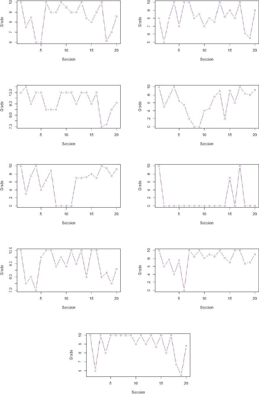
The following data, in Figure 1, corresponds to a class taught by one of the authors of the present work. In this class, twenty sessions were evaluated through homework’s graded from 0 to 10. The plots correspond to 9 students who took this class, and we note that the values of each grade are not uniformly distributed, which would be the case if such values were independent.

The data above show that assuming a binomial distribution for the number of topics understood by a student is not always realistic. However, it might be the case that dependence grows very small with the understanding of each session, a situation which might reflect that the student eventually had to learn all the material from previous sessions, which they did not understand at first. This could be the situation presented, for instance, in the plots in positions (2,1) and (2,2). In this case a binomial model in the long-time scenario might be accurate.

With all the previous arguments in mind, we consider the case when the learning process has dependence not only on the present session, but also on every previous session. This implies that the probability of successfully learning the content of each session is varying over the time, according to some parameter which measures the influence that previously learned topics from previous sessions have in the present result. This also models the fact that students are accumulating knowledge across time, which helps them to understand in an easier way depending on whether or not they understood all or just some of the previous sessions.

We also assume that, however, after a sufficiently large number of successes or failures, the parameter which measures the influence of past topics will decrease and hence we prove that this results in an asymptotically binomial model for which quantities of interests can be approximated in a simple way.

The initial assumption removes the restriction imposed by the Markov property and provides a different approach in the modelling of learning processes. Our model considers the following assumptions:

Assumption 2 implies that each student is isolated. The influence of the interaction between the students may be considered for future work under additional assumptions on the dependence parameter ε. Nevertheless, this assumption applies, for instance, to situations like homeschooling, tutorials, postgraduate studies, online classes, and introverted students.

In all this work, the parameter q is used a 1 - q. The reason for this is merely technical and it means that, in the case of a distribution supported in (0,1), 1-q intuitively measures how poor the quality of sessions was, i.e., the poorer the quality the more difficult it will be for the student to understand the session.

As we will see in one of our simulations, if the distribution F is supported in the whole real line, the value of q might be negative meaning another scale to denote low quality sessions.

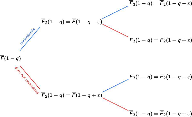
The event in which the student understands the first session has a probability given by F¯(1-q), where F¯ :=1-F.

From the second session until the end of the course, if the student understood session j, they understand the next one with probability F¯j+11-q≔F¯j1-q-ε. Here F1 refers to the initial distribution F and each Fj for j≥2 is constructed conditioned on the result of all the previous j-1 sessions.

Similarly, if the student did not understand session j, they understand the next one with probability Fj+11-q≔Fj1-q+ε. These changes can be visualized in Figure 2.

Thus, the dependence parameter, defined in Assumption 5, helps us to keep track on how the results of session j influences session j+1. Whenever a student understands the session j, it is a little more likely that they understand the next one. An analogous situation occurs if the student does not understand session j. In the following sections we manipulate this model to obtain some results related to the distribution of the number of sessions that the student understands along the course.

3. Results and discussion

We let Y (j) be Bernoulli random variables defined as follows: For session 1, Y(1) is Bernoulli with parameter F¯(1-q) for the given initial continuous distribution F. For session 2, by the Law of Total Probability we have:

Given that the student understood session 1, the probability that they understand session 2 is given by:

Similarly, if the student did not understand session 1, the probability that they understand session 2 is:

It follows that (1) is equivalent to:

For the general setting, we denote by Fj the probability distribution such that:

Provided that F¯j-1x-ε and F¯j-1x+ε do not equal zero or one. In the equation above, pk≔PYk=1 for k>1 with p1=F¯1-q and F1≔F. Using this notation, we obtain:

Throughout the rest of this paper, we assume that 1-q±nε is such that 0<F1-q±nε<1, for each n. In the following result we derive a recursive expression for the probabilities {pm,1<m≤n}.

Theorem 1. The general expression for {pm,1<m≤n} reads:

Proof. See Appendix ∎

From this point on, we drop the notation F1 and write F instead.

We let Bn denote the number of sessions, not necessarily consecutive, from a total of n that the student understood. We are interested in the probability function of Bn, {P[Bn=k],0≤k≤n}, for which we consider the following particular cases.

Case 1: n=3 and k=0.

This is the case when the student understands 0 sessions out of 3. The probability reads:

Case 2: n=3 and k=1.

If student understand only one session (i.e., k=1), the probability is the sum of the following cases.

2.1. The student understands only the first session:

2.2. Student i understands only the second session:

2.3. And student i understands only the third session:

Note that the probabilities in cases 2.1 and 2.2 equal P[B2=0]F(1-q) and the probability of case 2.3 corresponds to P[B2=1]F(1-q+2ε). Hence:

Case 3: n=3 and k=2. If student understand two sessions (i.e., k=2), the probability is the sum of the following cases.

3.1. Student i understands the first and second sessions but not the third:

3.2. Student i understands the second and third sessions but not the first:

3.3. Student i understands the first and third sessions but not the second:

Note that cases 2 and 3 correspond to P[B2=1]F¯(1-q) and the first case equals P[B2=2]F(1-q-2ε). Hence:

Case 4: n=3 and k=3.

This is the case when student i understands all sessions. This probability is given by:

The recursive behavior observed in the probability function of B ₃ is generalized in the following theorem.

Theorem 2: Let n≥3 be an integer. The probability function of the random variableB3satisfies the following relations.

Proof. See Appendix ∎

Equations in Theorem 2 can be written as a single matrix equation. Let Bn→∈M1,n+1 be given by:

And denote by Mn∈M1,n+1 the matrix such that:

Using the notation above we note that Bn→=Mn⋅B→n-1, therefore:

Where: B0→=F1-q,F¯1-q. This representation is used for some numerical examples in the figure section.

The explicit distribution of Bn is not easy to obtain even in simple cases (such as the case when F is a uniform distribution). Nevertheless, in the following result we provide a simple asymptotic expression for this distribution.

Theorem 3: Let {pnk,k=0,1,…,n} denote the probability function of a Binomial (n,p) distribution, withp :=F¯(1-q). Supposen,ε are such that n2ε → 0 as n → ∞ and F is absolutely continuous with density f such that f is continuous at 1 - q, then:

Proof. See Appendix ∎

Theorem 3 says that for a sufficiently large number of sessions the dependence becomes less relevant, hence the number of sessions that each student understands behaves like a binomial distribution in which the occurrence of successes is independent. The convergence referenced in Theorem 3 does not imply, in general, the convergence between the means of Bn and the limit binomial random variable. However, in this case such convergence holds.

Theorem 4: EBnnF¯1-q→1 as n → ∞.

Proof. See Appendix ∎

Three numerical examples of the result above are given in Figure III (Appendix), where we note that both means, the simulated and the approximated one, behave similarly. On the other hand, the values of the quotient EBnnF¯1-q are mostly in the interval (0.98,1.02).

Estimation of the quality of the course q: It is possible to use the approximation in Theorem 4 to estimate the quality parameter q. This is stated and proved in the following result.

Theorem 5: Assume that F¯ has a continuous inverse function F¯-1 and set qn:=1-F¯-1EBnn . Then qn→q as n→∞.

Proof. See Appendix ∎

Example 1. For the data considered at the beginning of Section 2, we have 22 students taking the same course and we use their grades to determine whether they understood the lessons or they did not (we assume that grades equal or greater than 6 indicate the student understood the lesson).

The whole exploratory data indicated that the grades of students are not identically distributed and thus, we approximated the value of q for each one of these students using the result of Theorem 4 and the empirical estimator of EBn. The development of a statistical tool to test the goodness of fit from data may be an interdisciplinary option for future work. These results are presented in the table below.

The average of this estimations is 9.1. In the official instrument, made by the university, where the students grade the quality of the course, the same course was graded 9.6.∎

By Theorem 5 we have:

This estimation of q under this model is illustrated in Figure IV (Appendix) in plots (a) and (b), where we also consider a standard normal distribution (plots (c) and (d)). We note that the values of q in these examples provide a criteria to determine if the quality of the course’ sessions has been poor or not. For instance, as we see from the perpendicular dashed lines, q=1 implies a course in which the student understood just half the sessions, which might be considered as low quality course.

In Figure I (Appendix) q and simulate the exact distribution of Bn. Then we compare it to the approximating binomial distribution given in Theorem 3 for number of sessions given by n=10,30,60,100 (plots in blue, red, green, and purple respectively). The light line corresponds to the approximating binomial distribution while the dark line represents the simulated exact distribution. We see in these plots that the convergence to the binomial distribution is quite fast, and it grows faster when q = 0.5.

Our numerical examples show that the speed of convergence depends on the value of q, as it can be seen in Figure II (Appendix) q with fixed n and compare the exact distribution of Bn to the approximating binomial distribution.

Another point worth mentioning is that the distributions behave symmetrically with respect to q=0.5. In this case, the convergence to the binomial distribution is faster than in the other cases. In fact, the cases when q is nearly 0 or 1, present a slower convergence to the binomial distribution. This may imply that the dependence is stronger when the quality of the class is low or high.

4. Conclusions

In this work we present a model to study the behavior of the understanding of a student along several sessions of a course without interaction with other students. In particular, we study the case where the dependence between sessions is relatively small compared to the total number of sessions, as in seminars or panoramic courses. We obtained a recursive expression for the distribution of the number of sessions that the student understands along the course and showed that when the dependence parameter is small, this distribution has a binomial approximation. The speed of convergence of the approximation depends on the number of sessions and the quality of them. Even though this is a simple model, it can be fruitfully extended to consider many more situations, some of which we list below:

5. Supplementary Information

Appendix.

References

[1] Bower GH. Application of a model to paired-associate learning. Psychometrika. 1961; 26(3): 255-280. Disponible en: https://link.springer.com/article/10.1007/BF02289796
[ Links ]
[2] Busemeyer JR, Diederich A. Cognitive modeling. Sage; 2010.
[3] Cajueiro DO. Enforcing social behavior in an Ising model with complex neighborhoods. Physica A: Statistical Mechanics and its Applications, 2011; 390(9):1695 - 1703. Disponible en: https://www.sciencedirect.com/science/article/pii/S0378437111000501
[4] Chechile RA, Sloboda LN. Reformulating Markovian processes for learning and memory from a hazard function framework. Journal of Mathematical Psychology, 2014; 59: 65-81. Special Issue in Honor of William K. Estes. Disponible en: https://www.sciencedirect.com/science/article/abs/pii/S0022249613000862
[5] Coombs CH, Dawes RM, Tversky A. Mathematical psychology: An elementary introduction. 1970.
[6] Dufresne RJ, Gerace WJ, Leonard WJ, Mestre JP, Wenk L. Classtalk: A classroom communication system for active learning. Journal of Computing in Higher Education. 1996 Mar; 7(2):3-47. Disponible en https://link.springer.com/article/10.1007/BF02948592.
[7] Estes WK, Suppes P. Foundations of stimulus sampling theory. 1974.
[8] Huang YM, Huang TC, Wang KT, Hwang WY. A Markov-based Recommendation Model for Exploring the Transfer of Learning on the Web. Journal of Educational Technology and Society. 2009; 12(2):144-162. Disponible en https://www.jstor.org/stable/jeductechsoci.12.2.144.
[9] Klemm K. Nonequilibrium transitions in complex networks: A model of social interaction. Physical Review E, 2003; 67(2). Disponible en: https://journals.aps.org/pre/abstract/10.1103/PhysRevE.67.026120
[10] Laming F, Straile R. Photoresist cleaning. Journal of The Electrochemical Society, 1973; 120(2):292.
[11] Lee YA. Third turn position in teacher talk: Contingency and the work of teaching. Journal of Pragmatics. 2007; 39(6):1204 - 1230. Disponible en: http://www.sciencedirect.com/science/article/pii/S037821660600227X.
[12] Levine G, Burke CJ. Mathematical model techniques for learning theories. 1972.
[13] Li C, Liu F, Li P. Ising model of user behavior decision in network rumor propagation. Discrete Dynamics in Nature and Society. 2018 Aug; 2018:1-10. Disponible en: https://www.hindawi.com/journals/ddns/2018/5207475/.
[14] McCroskey JC. Classroom consequences of communication apprehension. Communication Education. 1977 Jan; 26(1):27-33. Disponible en: http://dx.doi.org/10.1080/03634527709378196.
[15] Nakayama S and Nakamura Y. A fashion model with social interaction. Physica A: Statistical Mechanics and its Applications. 2004; 337(3):625 - 634. Disponible en: http://www.sciencedirect.com/science/article/pii/S037843710400113X.
[16] Ostilli M, Yoneki E, Leung IXY, Mendes JFF, Lió P, Crowcroft J. Ising model of rumour spreading in interacting communities. University of Cambridge, Computer Laboratory; 2010. UCAM-CL-TR-767. Disponible en: https://www.cl.cam.ac.uk/techreports/UCAM-CL-TR-767.pdf.
[17] Restle F, Greeno JG. Introduction to mathematical psychology. 1970.
[18] Richmond VP. Communication in the classroom: Power and motivation. Communication Education. 1990 Jul; 39(3):181-195. Disponible en: http://dx.doi.org/10.1080/03634529009378801.
[19] Roberts FS. Discrete mathematical models, with applications to social, biological, and environmental problems. 1976.
[20] Stauffer D. Social applications of two-dimensional ising models. American Journal of Physics. 2008 Apr; 76(4):470-473. Disponible en: https://doi.org/10.1119/1.2779882
[21] Wickens TD. Models for behavior: Stochastic processes in psychology. WH Freeman & Co Ltd; 1982.
text new page (beta)
English (pdf)
Article in xml format
Article references
Send this article by e-mail
Cited by SciELO