


 text new page (beta)
 English (pdf)
 Article in xml format
 Article references
 Send this article by e-mail
 Cited by SciELO
  Similars in
SciELO
Similars in
SciELO 
 Permalink
1. Introduction
1.1. Form-finding versus the Force Density Method
Most unstressed 2D and 3D tensile bar structures are kinematically indeterminate. As a result, their final equilibrium configuration geometry, i.e. the position of the nodes, is a priori unknown. The search for an initial shape compatible with a set of loads and constraints is termed form-finding .
A tensile structure can be seen as a materialization of a 3D funicular . This is also the case for masonry structures when a Limit Analysis approach is used, as the problem here is also based on the funicular concept. The link between form-finding methods and funicular analysis is therefore straightforward.
The Force Density Method, FDM (Linkwitz & Schek, 1971; Schek, 1974) was developed in the 1970s as a form-finding procedure for cable tensile structures (Grundig, Moncrieff, Singer, & Ströbel, 2000).
FDM was selected for this research due to four main considerations: (1) It manages equilibrium equations in a totally direct way, and is therefore especially suited for a funicular solution; (2) equilibrium equations are linearized, which simplifies the numerical process, even though an iterative analysis is usually needed; (3) no pre-sizing is required for this method; this is a crucial question for many approaches and particularly for the two new applications addressed; and (4) the three equilibrium equations are uncoupled , an important property that will be exploited here.
1.2. Funicular analysis versus masonry structures
Funicular analysis refers to the use of a 2D or 3D funicular as an analytical tool at any stage of the analytical process. Additional assumptions would also make it a design tool, as in the case of masonry structures Limit Analysis . The funicular concept is not restricted to linear elements, e.g. cable structures, but could also be applied to surface elements, e.g. for creating membranes.
This paper will describe a wire frame model, either linked with linear elements or representing membrane discretization, with special focus on the case where there is only tension or internal compression force; although some procedures are valid for both tension and compression if proper constraints are considered.
The first application of Limit Analysis theory (Kooharian, 1952) for the analysis and design of masonry structures has being notably expanded and consolidated (Heyman, 1966, 1969).
The assumptions inside this frame are: (i) Constitutive equations are rigid-plastic, with no tensile strength but infinite compressive strength, (ii). Friction between the voussoirs is sufficient to prevent failure due to sliding between them; (iii). Stability is only considered inside a rigid multi-body model and according to the first assumption (i).
A high span or great depth of the mortar between voussoirs would make the first assumption impossible, (i) Assumption (ii) can be checked a posteriori. The validity of assumptions (i) and (iii) run quite parallel. Nevertheless, in the majority of cases, the said assumptions can be applied, and then funicular analysis is really simple: the structure is safe (Lower Bound Theorem or Safe Theorem ) if at least one thrust-line, i.e. a funicular , can be traced inside the geometrical boundaries of the structure (Poleni, 1748). This is in fact quite an old supposition, but once it has been included within the framework of Limit Analysis its level of reliability becomes clear. The use of form-finding methods for funicular analysis is therefore totally justified.
The question of adding constraints for selecting a particular funicular has been approached in different ways. One of the first was to use linear programming (Livesley, 1978). In the Force Network Approach, FNA (O'Dwyer, 1999) the equilibrium path is fixed in one plane, in this case in the horizontal one, i.e. the projection of the 3D funicular in this plane therefore the thrust is fixed. Afterwards, the ordinates of the funicular target are obtained by linear programming. This method limits its application to the case where loads are perpendicular to the plane where the equilibrium path is fixed (usually the horizontal one), which is its most important drawback.
The idea of fixing the 3D funicular projection into a plane together with thrust in the corresponding directions had been proposed for cable tensile structures, and is known as the Grid Method , GM (Siev & Eidelman, 1964). The condition of vertical equilibrium makes it possible to obtain coordinates perpendicular to the grid, giving rise to a system of linear equations. GM was also limited to the case of load perpendicular to the grid. A similar approach was used in fixing the horizontal path of the funicular in a grid together with thrust. Equilibrium is resolved iteratively node by node (Berger, 1996).
FDM is especially suited for fixing the funicular path in one plane, as the equilibrium equations in three perpendicular directions are uncoupled . As was pointed out above, this property is one of the main advantages of the method.
Thrust Network Analysis , TNA (Block, Ciblac, & Ochsendorf, 2006; Block & Ochsendorf, 2007; Block, 2009) is strongly connected with FNA , but adds parallel handling of the reciprocal or dual figure to horizontal projection, i.e. the force diagram, and the use of the FDM .
The Analytical , A-FDM , and the Numerical method , N-FDM , are both described in this article. They are based on parametric application of the original FDM for obtaining funicular solutions, and were independently proposed by the authors (Cercadillo-García & Fernández-Cabo, 2010; Cercadillo-García, 2014).
1.3. Funicular analysis versus preliminary design
Preliminary design refers to the application of a 2D or 3D funicular for selecting the initial shape of a structure, assuming that a funicular shape leads to high structural efficiency.
The use of physical models to support preliminary design has been present throughout the history of construction. Hanging models have been used to trace the funicular . The well-known case of Antoni Gaudí may constitute the highest expression. In the 1960s and 1970s physical models were replaced by computer models.
Tensile structures needed computer models, and funicular analysis is now consolidated as an independent area. Together with other new architectural lines such as using free (i.e. organic ) form s. Computational improvements are promoting and challenging this working line (Kilian & Ochsendorf, 2005).
1.4. Funicular analysis versus the parametric method
Parametric refers in part to the parametric capability of tools used in symbolic computation in e.g. Maple ®; but it mainly describes to the nature of the proposed method, such as searching for a specific funicular , which is parameterized in terms of independent variables.
This paper presents a new method, the Parametric Force Density Method , for tracing a selected 2D or 3D funicular (Cercadillo-García, 2014). This method is developed in different ways: Analytical , A-FDM , and Numerical , N-FDM , extensions of FDM . The application of the methods to the fields of masonry structure and preliminary design are specifically addressed.
The mathematical software Maple ® is used to implement structural algorithms, and its capability to work symbolically is especially important. AutoCAD ® is used as a graphical and geometrical tool. Maple ® results are exported to AutoCAD ® compatible files, and both environments are linked in real time.
2 Method
2.1. Original FDM
FDM states the problem for a pin-jointed structure of straight bars. Let m be the number of bars, n the number of total nodes of the structure, n f the number of free or unconstrained nodes, and n c the number of fixed or constrained nodes. Load, p i , is located at the nodes. For the node number i , their Cartesian coordinates are (x i, y i, z i ).
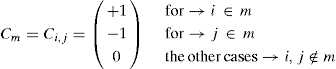
The Branch-node matrix was known originally as the Incidence matrix , [C ]. Its rows are linked with the branches or bars, ordered from 1 to m , and its columns are linked with the nodes (but dividing the free and constrained nodes, as will be shown). If i (m ) is the initial node number of the branch m and j (m ) its final one, with i (m ) < j (m ), the components of [C ] are defined by:
 (1)
(1)
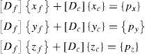
The matrix [C ] is partitioned in two matrices, containing free nodes and fixed ones separately, [C ] = [C f ] + [C c ]. Using a compact form with curly brackets {...} for a column vector, and square brackets [...] for a matrix, the equilibrium equations then take the form:
 (2)
(2)
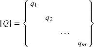
where [Df]=[Cf]t[Q][Cf] and [Dc]=[Cf]t[Q][Cc],[Q] is the Diagonal matrix associated with vector {q}t=〈q1,...,qm〉, and q k are the Density force values , i.e. the relationship between the force and the length of the bar number k:qk=tk/lk.
 (3)
(3)
If the loads are known and the q k values are established a priori, the only unknown variables in Eq. (2) are the coordinates of the free nodes (x f, y f, z f ). Eq. (2) is linear, and the number of equations is equal to the number of unknowns. For the case when all q k values have the same sign (i.e. with all the bars under tension or compression), the matrix [D ] is positive and the values of (x , y , z ) can be univocally determined. [D ] is usually termed the Force Density or Connectivity matrix . Linear equilibrium equations are uncoupled , so the coordinates (xf,yf,zf) would be obtained independently. This is an important fact (as will be shown in Eq. (4)).
The idea of including the relationship between force and bar length in one term, i.e. the idea of defining q k as a variable, was pointed out at the beginning of the XX century, when this variable was termed the Tension coefficient (Kotter, 1912; Southwell, 1920). The method of Tension coefficients (the term Tension coefficient is used instead of Force density ) addressed the analysis of pin-jointed frames, and it is not form-finding . It was considered to be especially suited for three-dimensional frames (Parkes, 1965).
2.2. An alternative algorithm for the proper management of constraints
Instead of referring to the number of nodes (total, free or fixed), the variables must be the number of degrees of freedom, DOF. According to this, e.g. for direction x , n x refers to total number of DOF, n fx to the number of released DOF and n cx to the number of constrained DOF. For the three directions, the next equations define the number of free and constrained, DOF, where n x = n fx + n cx (and the same for the other two directions). Eq. (4) then has to be written, as a partitioned matrix (for directions y and z the relations are symmetrical, simply by replacing x with the new direction):
 (4)
(4)
Eq. (4) assumes (i.e. in the original proposal) that free nodes are released in their three components and that the same is the case for the fixed ones. But this assumption notably limits the proper management of constraints, an important question that is especially important due to the uncoupled character of Eq. (4). For partial constraints the branch matrices and [C c ] must be independently established for the equilibrium in each component.
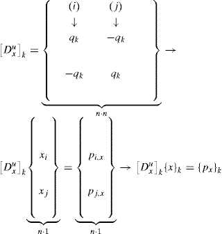
The formulation of the equilibrium equations (Parkes, 1965; Pellegrino & Calladine, 1986) permits one alternative for direct assembly of the matrices [D f ] and [D c ]:
 (5)
(5)
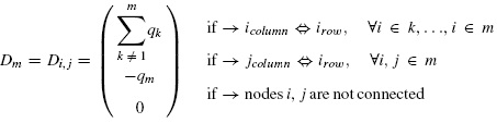
Rows are linked to the free nodes and columns are linked to the global nodes (i.e. the free and constrained nodes), their members are the negative Force density value of the bar or branch m when there is a relationship between the first node i (m ) in a row with the final node j (m ) in a column. If a free node, where actual equilibrium is sought, is in both row and column, the component of the matrix belongs to the sum of all the Force densities of the branches to which that node belongs, and finally, it will be zero if the nodes in a row and column are not connected.
Therefore, after determining the Connectivity matrix or Force density matrix , [D ], it is possible to resolve the equilibrium position of the free nodes, n f , and thus the geometry of the system:
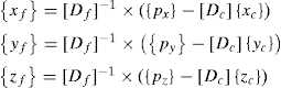 (6)
(6)
The Force density matrix would be directly assembled once connectivity is established in some way (Vassart & Motro, 1999), and not necessarily by means of the Branch-node matrix (Schek, 1974). This is relevant because the next alternative procedure, as will be shown, directly connects with the typical theory of structures.
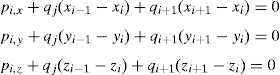
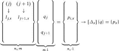
Considering the equilibrium at node i where the bars or branches j and j + 1 are connected; p i, x and p i, y are the external loads at that node i and t j and t j+1 the resulting stresses or internal forces at the j and j + 1 branches respectively.
Sign criteria are defined in Figure 1, and the three equilibrium equations are:
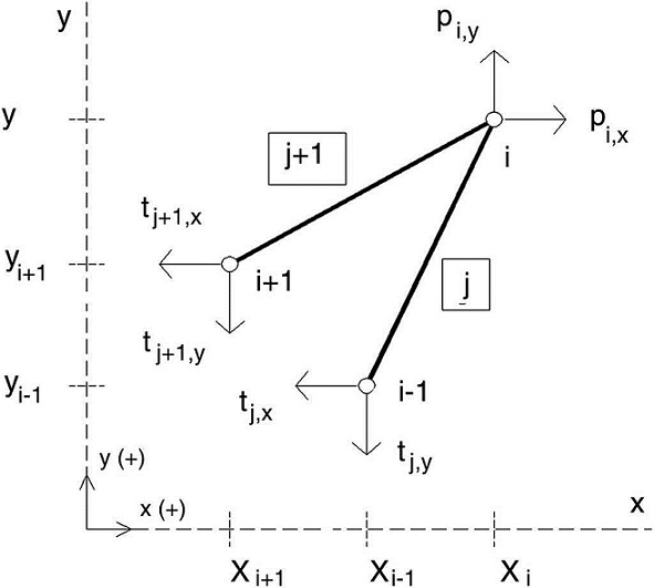
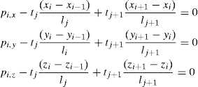 (7)
(7)
Eq. (6) brings together the internal forces t and the length of the bar l in one variable, the Force density (e.g. qk=tk/lk).
 (8)
(8)
If the constraints are not yet defined, i.e. if the structure is free-standing, the equilibrium equations are therefore established for the whole nodes:
 (9)
(9)
where the contribution for a bar k , joining the nodes i and j , with i < j , to the unconstrained Force density matrix , at the equilibrium at x axis, is (the order of the vectors being {p x } and {x } is consecutively from 1 to n ).
By summing the contribution of all the bars, the unconstrained Force density matrix is obtained to Eq. (10):
 (10)
(10)
But in fact, only one unconstrained Force density matrix , [Du], is needed for the whole problem, as:
 (11)
(11)
This is the same process that is used for assembling the Stiffness matrix by means of the Direct stiffness matrix . The application of the boundary conditions is understood as a further step for getting a solution, as it is the application of a particular load. The possibility of using basic figures of the theory of structural analysis is desirable from a conceptual point of view.
A Connectivity matrix is of course needed. But the Branch-node matrix includes topology as well as the boundary conditions; and generally speaking, three different matrices are needed. In this alternative, the topology is defined by a unique matrix in all cases; and another matrix (or three vectors) manages the boundary conditions, and therefore these can be modified very easily and independently. The constrained Force density matrix must then be automatically generated.
For instance, the connectivity of the two bars depicted in Figure 1 can be stored in a typical connectivity matrix, IF , according to:
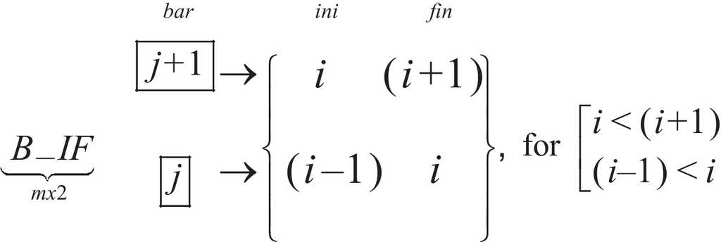 (12)
(12)
An algorithm (in pseudo-code) for assembling [Du], is (remembering that m is the total number of bars), where D _t means the n ·n matrix assembly, q [k ] represents the element k of vector q and B_IF[i,j] the element of the matrix B_IF corresponding to row i and column j:
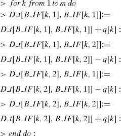 (13)
(13)
Constrained matrices [Dx],[Dy],[Dz], can be automatically generated from [ Du ] by means of three auxiliary vectors ({gx},{gy},{gz}), that define the active DOFs for the three axes, e.g. for a system with four nodes, a vector {gx}=〈0111〉t means that the displacement x of the first node is constrained, while the other three remaining nodes are released. With this information, the first row of the unconstrained matrix [ Du ] can be removed to obtain the final constrained one, [D x ].
The idea of assembling the whole unconstrained matrix [ Du ] after deleting the invalid rows has been also used (Xi, Xi, & Qin, 2011). This procedure is easy to implement (the authors have applied it using Maple ®).
The use of partially constrained nodes is now possible and easy to manage, a crucial question. Eq. (4) can be re-arranged in other ways. One alternative is to consider the Force densities as variables.
For the case depicted in Figure 1 (and similarly for the other matrices):
 (14)
(14)
And for the whole structure (d = 2, to 2D and d = 3, to be considered a tridimensional system), although it would be possible to combine all next three equations in a single one, to manage constraints it is useful keep them independent (or sometimes in a group of two):
 (15)
(15)
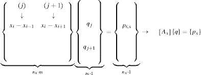
Matrices [A ] used to be termed as Equilibrium matrices , even though they are not exactly the typical Equilibrium matrix of structural analysis, which can be directly obtained from Eq. (14) by grouping terms of type (xi−xi−1)/lj. An educational implementation of the typical Equilibrium matrix from Maple ® can be seen in (Fernández-Cabo, 2012). Another interesting alternative which other authors have pointed out, is to consider the length components as a datum (Heam & Adams, 2006).
For the case shown in Figure 1, where lj,x=xi−xi−1 and lj+1,x=xi−xi+1 (note that these scalars, even though they are finally projections of the length of the bars along three global axes, have signs, and that being positive or negative leads to different results).
 (16)
(16)
For the whole structure:
 (17)
(17)
In all cases, the authors adopt the procedure of first assembling a common unconstrained matrix before using vectors to add constraints and remove non-active DOFs.
And of course, a mixed procedure that combined variables is possible. As will be shown in the next sub-section, the following combination is of special interest ({q }, [Δ]) and ({q }, [x ]). This can be made quite straightforward in Maple ®, as the unknowns are set each time for the same set of equilibrium equations.
Using Maple ® it is also easy to add additional constraints, e.g. geometrical ones. This will be shown in the examples, as it is of particular interest.
Using this general framework, two specific procedures, one Analytical , A-FDM , and other Numerical , N-FDM , will be explained in the next sub-sections. These two methods do not complete all the possibilities, but illustrate two research techniques.
2.3. The Analytical parametric procedure: A-FDM
The Analytical procedure is based on (Vassart, 1997; Vassart & Motro, 1999; Zhang & Ohsaki, 2006; Zhang, Ohsaki, & Kanno, 2006).
As was pointed out above, when all the q k values have the same sign, i.e. there are only tensions or compression, the matrices [Dx],[Dy],[Dz], are non-singular (and are termed regular ) and the system of equations is determined, leading to a unique solution, where rank[Dx]=rank[Dy]=rank[Dz]=n, and det[Dx]=det[Dy]=det[Dz]≠0.
Work in the field of tensegrities pointed out that when tensions and compressions exist the matrices [Dx],[Dy],[Dz], tend to be singular (Vassart & Motro, 1999; Tibert & Pellegrino, 2003). constraints have to be added to gain a particular solution. Another possibility is to add constraints to reach an undetermined solution, i.e. a parametric one.
In general terms, the use of FDM , in any of the alternatives described in Section 2.2, leads to the solution of a linear system (sometimes iteratively) of the form (Eq. (18)), where the matrix [M ], collecting known factors, can be square or rectangular; {b } is a vector of known data; and {a } is the vector of unknowns:
 (18)
(18)
When the matrix [M ] is square and non-singular a unique solution exists, so that rank[M]=n, and det[M]≠0.
Otherwise the system is undetermined, where infinite solutions exist and so rank[M]<n, and det[M]=0. But this is akin to saying that a parametric solution exists.
The parametric form can be obtained by transforming the corresponding augmented matrix 〈[M]e|[d]e〉, into its row-echelon form , (rank〈[M]e|[d]e〉 <n, and det〈[M]e | [d]e〉=0:
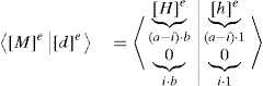 (19)
(19)
where [H]e is the corresponding row-echelon matrix , and can also be the Hermite or reduced Row-echelon matrix , which has the important property of being unique.
According to linear algebra, the system is consistent and undetermined when [H]e is not square, with necessary means that rank [H]e < b), and the number of parameters, p , are equal to p=b−rank[H]e.
The use of the row-Echelon matrix to reach a parametric solution , for the case of statically undetermined structures, can be seen in (Guest & Calladine, 2000). This work is totally linked with (Pellegrino & Calladine, 1986). Here the redundant forces are the parameters that express the whole solution of the problem.
The algorithm for Analytical parametric control is described below, and to date it has only been successfully applied to loads having the same direction, such as dead load, which is obviously an important limitation.
STEP 1. Define the system of parallel load by means to any mesh Γ perpendicular to the system (along a line in 2D, Γ1D, or in a plane for 3D, Γ2D).
STEP 2. Define the load or, in the case where the difference between the reference and final configuration it is not relevant (as is the case for masonry structures or preliminary designs) the load ratio (i.e. a load vector {p } proportional to the actual one).
STEP 3. Define the general unconstrained matrix , [ Mu ].
STEP 4. Apply boundary conditions, the degrees of freedom for each node/direction and remove the rows of [ Mu ] corresponding to fixed nodes, obtaining the general matrix [M ], for the theoretical matrix equation, [M]{a}={b}. For a specific method, as is the case of [A x ] or [Δx] in 2D, and the matrices, [Ax],[Ay] or [Δx],[Δy] in 3D. It is also possible to combine variables of type [A ] and [Δ]. When using [Δ], if all the terms in the linear equations are divided, at both sides of the equation, e.g. by the span of the structure, the shape is controlled in a non-dimensional way, i.e. the proportion is finally the variable, and not a specific set of coordinates (Andreu, 2005).
STEP 5. Obtain the Echelon matrix (or reduced Echelon matrix ), [H]e, to give the solution. When the matrix [M ] is not square, firstly it will be necessary to determine the augmented Row-echelon matrix , 〈[M]e|[d]e〉.
STEP 6. The designer could add geometrical constraints in order to reduce parameters, p , and improve management of the problem, when too many parameters have to be defined, p=b−rank[H]e. The system is undetermined when rank[H]e < m (less than the number of bars), and therefore the number of parameters necessary for one valid solution, should be equal to p=m−rank[H]e.
STEP 7. Impose the boundary conditions on the original unconstrained equation [Dy]{y}={py} to 2D or ([Dz]{z}={pz} to 3D) as a function of the selected parameter/s, which finally gives a parametric representation of the whole geometry.
STEP 8. A specific funicular can be draw by other computer tools, such as AutoCAD ®, which offers easy visualization of the whole geometry or set of admissible funicular .
Notice that this method is especially suited to the case where the geometry of the structure is known, and therefore the load vector can be defined at the beginning of the process. This is particularly so for analysis of masonry structures.
Supposing one bi-dimensional arch/cable with both ends totally fixed, if the Force densities were known, the matrix [M ] is square and non-singular . If Force densities are taken as variables, the difference between the number of bars, m , and the number of nodes, n , is always one, m = n − 1, which means that the whole set of admissible funicular is controlled with just one parameter, p .
For a general 3D case, the number of parameters can be huge. One way to reduce this number is to keep in mind that if an arch/cable is contained in a plane but placed in space, the whole set of admissible funicular is again controlled with just one parameter. This can be very useful when defining the mesh Γ2D . The other practical way of reducing the number of parameters, as was pointed out in the algorithm, is to add geometrical constraints (see Section 3 for additional details and examples).
2.4. The Numerical parametric procedure: N-FDM
Schek (1974) uses the general theory of optimization to resolve the question of applying the FDM with additional constraints, e.g. the length of a set of branches of their stresses. But from a practical point of view, this implementation can be extremely complex.
As an alternative, the forces (or lengths) of each bar k are regularized to the average value, tmed (or lmed), by every iteration as an iterative process (Dansik, 1999).
In the case of length regularization, the new Force densities at iteration (r + 1), qk(r+1), are obtained from the previous force at iteration (r ), and the length of the bar k at iteration (r+1), lk(r+1), which is has to be lmed(r):
 (20)
(20)
The Multi-Step Force-Density Method with Force Adjustment , MFDF , is based on the previous one but with regularization of forces. This method is used to adjust the Force densities , depending on a uniform value for internal forces (Sánchez, Serna, & Morer, 2007).
At iteration (r + 1), the force densities , qk(r+1), are recalculated as function of the force adjustment coefficient, fk=tk(r)/T, as the relationship between the element force, tk(r) and the desired uniform internal net force, T .
 (21)
(21)
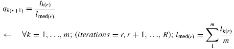
The Numerical method , N-FDM , seeks convergence to equilibrium by regulating the length of each bar k , lk, ∀k=1...m to a target value, lk,target, imposed a priori.
The Force density for the new iteration, qj,new, is written as a function of previous force, tk,old and target , lk,target:
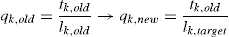 (22)
(22)
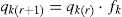
The algorithm is easier to use and without recalculation of forces as tk,old, it thereby only depends on the Force density , qk,old, and length, lk,old, of the previous iteration:
 (23)
(23)
This can be done not only for a bar k but also for a set of bars (let c be the number of constraints) and choosing a different target for each bar of the set i.e. Eq. (24).
As in any other optimization problem, only a maximum set of constraints can be imposed in each case. In large systems it can be very difficult to know in advance whether the selected constraints (selected a priori) will lead to a solution with convergence or not. But in practical terms it is very easy and quick to select a group of constraints and verify the convergence of the problem.
 (24)
(24)
When dealing with length, it is a good strategy to apply the constraints at the boundary end. Theoretical study of convergence is beyond the scope of this paper.
How is this specifically applied in the cases of masonry structures and preliminary design? Assuming that the bars can be considered inextensible (as this paper centres especially on masonry structures and preliminary design), the Numerical algorithm consists of:
STEP 1. The load vector {p } (which can be proportional to the actual one) is fixed a priori. There is no limitation on the direction of the loads (two or three components can theoretically exist), and therefore this method is more general than the Analytical one described above.
STEP 2. Define the length target/s vector, l target . In many cases it is convenient to use a scale factor, α ; where {ltarget}t=α⋅〈...lk,target lk+1,target...〉t, as it adds to the control of parametric solution.
STEP 3. Impose boundary conditions (which can be non-symmetric) on the unconstrained equations: [Dx]{x}={px},[Dy]{y}={py},[Dz]{y}={pz}.
STEP 4. Obtain a first set of coordinates (x, y, z) using a constant value, e.g. qk=1, for all the branches. This corresponds, when all the bars are either under tension or compression, to a minimal surface, and this is a very robust starting point.
STEP 5. The length (in 2D) or the areas (in 3D) of the elements is forced iteratively according the algorithm shown in Eq. (23) in order to fulfil the target/s .
STEP 6. Other software graphic capabilities make it possible to view the set of possible solutions, the whole set of admissible funiculars, by manipulating the parameter value α .
STEP 7. Lack of convergence can be controlled again, by reducing the number of constrained lengths or areas and repeating the process until convergence occurs.
The process is simple and quick, and the examples in Section 3 will prove its utility. This method is especially suited for the case where the geometry of the structure is initially unknown. This is usually in preliminary structural design.
Although the Analytical A-FDM , and Numerical method , N-FDM , could be combined, an important question regarding application must be mentioned: In order to obtain geometry, which is finally always the target in a form-finding problem, the load vector {p } does not necessarily need to contain the actual values, as a vector proportional to them would be valid. This is because there are situations, such as in masonry structures, where the difference between the initial length of the bars (i.e. the reference configuration) and the final one (i.e. the final configuration) is negligible in practical terms. This is akin to saying that the bars are considered inextensible (Poleni, 1748).
3. A-FDM and N-FDM: results and discussion
The Analytical , A-FDM , and Numerical , N-FDM , methods are based on parametric implementation of the original Force Density method , FDM , to determine the funicular equilibrium as a set of possible solutions. Selecting a specific funicular is related to the assignment of particular restrictions in the design process.
A-FDM and N-FDM are implemented by using three specific tools: (1) Assembly of the unconstrained Connectivity matrix , [Du], (2) A combination of matrix and indicial notation in linear equilibrium equations, and (3) The use of mathematical software with symbolic capability (Maple ®).
The Analytical method , A-FDM , is used to check security in masonry. It has been described as the funicular analysis of two-dimensional masonry structures, establishing analytical relationships between families of geometries, through equilibrium equations as a function of the length components of bars or as a function of thrust .
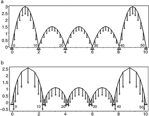
The Numerical algorithm method , N-FDM , is used as a design tool in funicular analysis . This method could be applied to determining the pressure line of an arch with constant thickness, which must be subsequently adjusted within the safety section to determine the equilibrium (e.g. Fig. 2).
N-FDM could be used in masonry for several arches (e.g. Fig. 3), even ones with arch supports at different heights. Only two end supports need to be fixed, as other supports work as sliding vectors and target , l target , is independently assigned according to span.
Both methods, A-FDM and N-FDM , will be used as a form-finding methodology for three-dimensional structures, and applied on built examples in the following sections.
3.1. Application in the preliminary design
N-FDM will be used as a design tool for two built structures: CNIT (The National Centre for Industry and Techniques , La Défense, Paris, France) and The PODS (Sports Academy , Scunthorpe, UK). Use with two examples with different geometries (with topological and additional constraints) will make it possible to validate the application of numerical technique to form-finding .
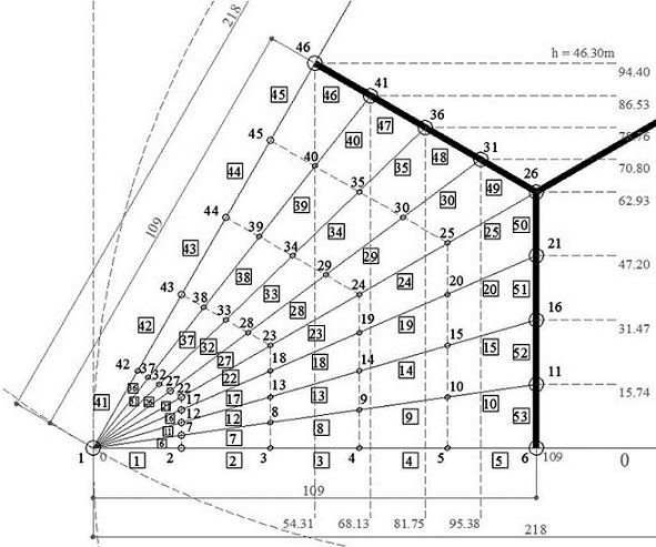
CNIT was conceived and designed by the French engineer Nicolas Esquillan , and it was built in 1956-1958. His proposal was for a vaulted reinforced concrete structure, consisting of a self-supporting double-shelled roof with spindles radiating from the three supports (vertices) on the floor: there are nineteen radial ribs on each symmetrical side of the equilateral triangle plan.
The shell has a radius of curvature ranging from 90 m to 420 m, and it covers an area of 900,000 m2. The ratio between its maximum height and front edge, which is located at a constant height at the three centroidal axes of the triangle, is approximately 1/4.5. The horizontal span measures 218 m on each face of the triangular plan and 46.30 m on the vertical span of the funicular shell.
Considering buckling forces, the shell of the roof is made of two thin surface layers, connected by cellular shear-force transferring diaphragms (prefabricated concrete walls) 9 m apart. The thickness of both surface layers, upper and lower, is only 170 to 240 mm (from top to support respectively) and the total thickness of the cross-section runs from 1910 mm at the top to 2740 mm at the support (Peerdeman, 2008).
The vault was designed to be built in three phases, starting with the first three waves on the ridge side, followed by waves 4 to 6 and finally waves 7 to 9 on the edges of the facades.
A remarkable part of the shell structure forms a tensile cord on each edge face. This function is below ground level to counteract outward thrust forces at each support. Due to the underground entrance and service shafts, the cord needed to be lower at the middle, forming a trapezoidal shape with two bending points. Horizontal tensile cords are anchored in the ground (Balency-Béarn, 1958).
Self-weight is the dominant load and radial ribs transmit the load, roof and dead load directly to supports. The final geometry is the consequence of assimilating each structural radial rib to the funicular (in the reverse direction) subject to the said load, designing a balanced system: the ribs work under compression while the straps on the façade are under traction.
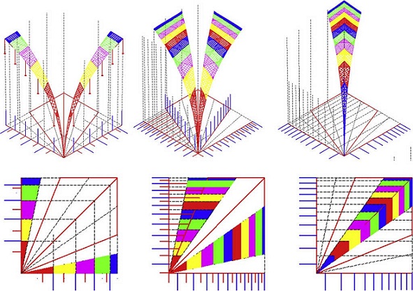
The topology is drawn in one third of the plan view due to its obvious symmetry, where the ribs are a set of branches connected by nodes (Fig. 4).
The edge nodes and the x , y coordinates of the internal free nodes are known.
Load is calculated depending on the attributed shell area, as a polygonal surface (Fig. 5), where a proportional section of the diagrams and the radial rib are added at each node. The final value depends on the total amount of concrete (m3), taking into account the weight for steel (2500 kg/m3). The number of radial ribs drawn, as a sum equal to 9, does not match the actual one, a total of 19. This is not considered relevant because funicular analysis is solely based on the attributed nodal area (Fig. 4).
There is only gravitational (vertical) load at each node. This is implies zero value in the other two directions, {p1,x}t=〈0〉1...46,{p1,y}t=〈0〉1...46. The Numerical algorithm method , N-FDM , could be used subsequently to verify and analyze the behaviour of the geometry obtained under the load states in other directions, such as that due to wind action.
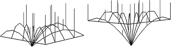
First equilibrium geometry (Fig. 6), is achieved thanks to the original FDM equations (Eq. (8)), assigning arbitrary and uniform force density values on bars, e.g. {q}t=〈1〉[1]...53].
The Numerical method , N-FDM , makes it possible to obtain the funicular that meets the geometrical constraint: horizontal thrust in the key (Fig. 7).


Radial ribs are classified into families from both sides of the central rib, which creates the symmetry of the plan view. The Numerical algorithm (Eq. (23)) regularizes the lengths of the bars for each family of radial ribs to the same target , l target , iteratively until convergence to the desired equilibrium is achieved. This process is repeated until the geometry has assimilated to the funicular with the horizontal tangent at its highest point. Nodal load is recalculated according to the discretization and attributed area in each new iteration.
For all families of radial ribs, it holds that the relationship between the projection, B , and target length, l target , is assimilated to the value, B/ltarget≈4.513, and the ratio between real length, L , and projection, B , resembles L / B ≈ 1.11.
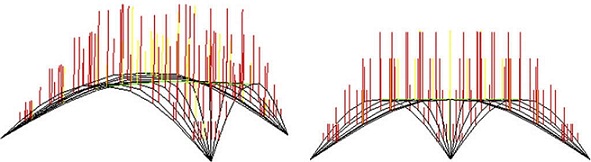
The Numerical algorithm , N-FDM , was programmed in Maple ®, where different and consecutive geometries are displayed in real time. The overall geometry is completed, to be graphically resolved by the drawing software of AutoCAD ®. Figure 8 shows coloured lines representing the gravitational loads at each node, according to recalculated values from Maple ®.
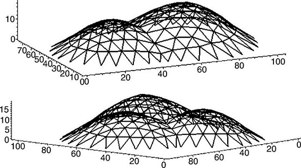
N-FDM is also applied as a design tool to The PODS Sports Academy , by Buro Happold , which opened to the public in the summer of 2011. The project has five shells of different sizes (the largest span measures 65 m and the smallest span is 15 m, across the diagonal) covering spaces for swimming pools, badminton courts, a gym, a dance studio, a coffee shop and a nursery.
The geometry is defined as a self-weighted triangular mesh in timber, and each interface stems from a steel arch beam, curved along the vertical plane and supported on columns along its entire length. The pattern of the geodesic mesh is similar to the spherical icosahedron , configured in hexagonal modules with a single pentagon on top. Edge nodes are fixed on the floor. Only compression stresses exist, but nodes and connections are designed to resist possible bending moments and shear forces.
Design efficiency is achieved through a process of optimization where the minimum number of nodes for equilibrium is determined, and regularization of the lengths for the maximum possible number of branches per dome is obtained by programming Dynamic Relaxation form-finding technique with Tensyl ® , SMART Software solution software (Harris, Gusinde, & Roynon, 2012).
The model could be analyzed and optimized by applying the Numerical method , N-FDM , replacing the Dynamic Relaxation method used by Buro Happold . As the conclusions have already been drawn, it is possible to proceed in reverse order: Defining, verifying and validating an optimum topology, creating a prototype arising from imposed constraints and boundary conditions relating to the original geometry.
For the initial research the total number of shells was simplified to two or three pieces, but keeping the topology, i.e. triangular frames and boundaries, with interface arcs (graph in green) and fixed nodes on circular edges. The internal nodes are set free, but interface nodes have only been allowed freedom along the vertical plane, i.e. in double geometry (Fig. 9), as they are fixed in the x coordinate and free in the plane yz .

Initial geometry as a hanging chain model is found with the original FDM equations for {q}t=〈1〉[1]...[m], using an arbitrary and equal value of gravitational point load. As in previous example, when the N-FDM algorithm runs (in Maple ®), the vertical load may be measured in each new iteration, depending on the new attributed nodal area and the assigned cover and structural weight.
Increasing the force density value of the diagonal edges to qdiag-edge=20, regularization of the edge diagonal lengths (included circular edge rings) for a single target , ledge-target=8, is easily obtained (Fig. 10).
However, the assignment of a unique target to the internal branches of a single dome or for all the domes together involves losing volumetric identity and deforming the geodesic convexity of the pieces.
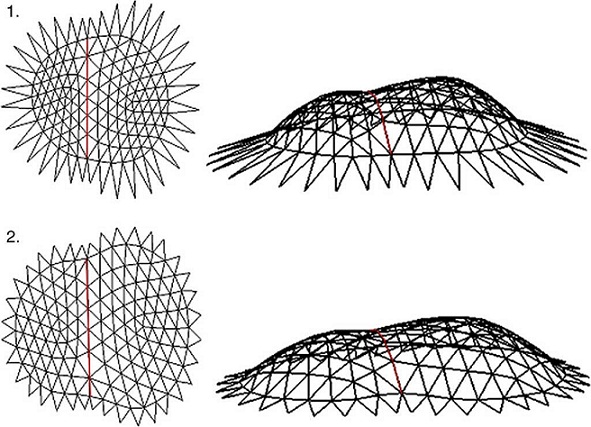
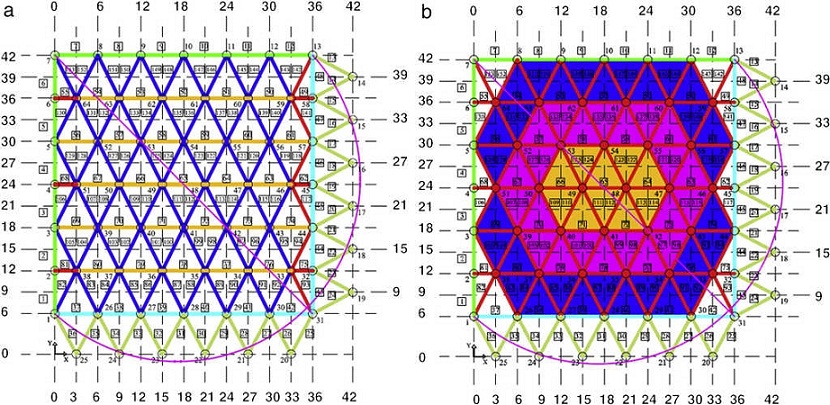
Two approaches (Fig. 11) were used successfully, where the diagonal branches in the interface dip (in magenta) and olive green branches are target to ledge-target=8, and the force density value for interface arcs (branches) is shown by {q}arc=〈8〉:
Regularization by assorted elements (Fig. 11a): Spiral ring bars in blue with the same value ledge-target=8, while the force density of internal diagonals (in red) is increased to qdiag-int=2.
Regularization according to assorted areas (Fig. 11b): The process is sequentially and incrementally inserted. The orange core with lcore-target=3, the intermediate strip (magenta) to lmedia-target=5.5, and lout-target=7 for the blue strip. White areas with an irregular grid must not be assigned any target for successful regularization.

Length adjustment is obtained in a high percentage of cases for both proposals if the pentagonal top and irregular frame of the first internal diagonals, next to the edge ring, are free of targets (Fig. 12).
Once the conclusions have been reached, the approach could be reversed: Determining the optimal topology pattern conformable to the original model, depending on the specific geometrical constraints and the desired target , e.g. homogenization of lengths as much as possible within the geometric equilibrium.
As a related topology, the basic pattern is set to square with two fixed edges, lateral right and bottom, and the remaining two, left and the top, are permitted freedom in the vertical plane parallel to length as interfaces (in green, Fig. 13).

Topological irregularities are minimized in the mesh, avoiding pentagonal order and reducing the disruption of the diagonal set up in zigzag only in the left and right side ends.
Validation of the square module will be conducted using two of the approaches discussed for the original geometry (Fig. 14):
Approach 1: Assorted elements. Branches are separated by type according to their location in the plan: horizontal (orange) and diagonal (blue).
Approach 2: Assorted areas. Branches are grouped into radial stripes and also marked in colours: the central core (orange), while the intermediate and edge rings are magenta and blue, respectively.
Lengths are regularized to a specific target depending on assorted elements or area analysis except in irregular frames, with horizontal branches in red (the first approach) and edge regions in white (the second approach, Fig. 15).
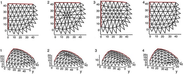
Convergence to equilibrium is then possible because of the uniformity of the rest of the plot. Gravitational load, based on attributed nodal area, is recalculated in each new iteration.
3.2. Application to masonry structures
The Analytical method , A-FDM , and the Numerical algorithm method , N-FDM , could be used for masonry. The case study is the ribbed vault of the Cathedral of Astorga (León, Spain).
The intersection between two pointed barrel vaults creates the ribbed vault , the skeleton of which consists of the cross ribs which join at the keystone. The bays in the roof are known as severies .
Some researchers doubt the structural role of the ribs , considering them to be purely decorative. However, it seems proven that the ribs are the frame of the vault and support the severies at first, after the removal of formwork and being placed under stress. They are also the essential element in creating the funicular of this geometrical design (Zaragozá-Catalán, 2008).
The Ribbed vault (or Ogive vault ) was the main structural element of Gothic architecture. It was developed from the late 11th century and in many cases was used until the XV-XVI century (late Gothic) or in adapted form in the Gothic Revival in England during the 19th century.
Construction of Astorga Cathedral, which is pre-Romanesque, commenced in Gothic style towards the year 1471. It is linked to two architects, father and son, John and Simon of Cologne. However, the southern front and two chapels are in Renaissance style, the main facade is baroque and was built during the eighteenth century, and is also has a neoclassical cloister. The Starry vault and ribs all with the same curvature is attributed to Rodrigo Gil de Hontañón. It was built in the sixteenth century, from 1550 to 1570.
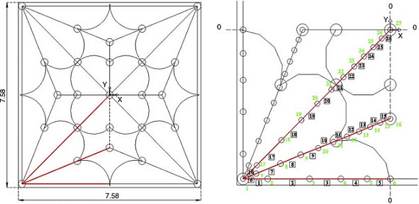
The cathedral vault has a square plan with sides 7.58 m long, and it is 5.14 m, high at the central key above the plane of imposts. Each of the quadrants is plotted with the cross rib flanked by a pair of tiercerons located on the bisector of the angle between the rib and two side arches , and ornamental arches are drawn tangent to each other.
Cross ribs , tiercerons and side arches draw the same radius of curvature, and the central key is slightly higher than the secondary and side keys (Palacios-Gonzalo & Martín-Talaverano, 2012).
The ribs are discretized as a set of branches with load points at the nodes. The symmetrical plan makes it possible to take only one reference, as half a quadrant may be drawn with a cross rib , a tierceron and a side arch (Fig. 16).
The gravitational load is determined according to the weight of the vault and a constant thickness. An equal area is attributed to all of the nodes, based on the uniform distribution of the severies . Final discretization implies a different projection of the lengths per branch. The colour differences here only indicate adjacent areas (Fig. 17).
Nodes, n f , are free on the vertical axis, and known for x and y , except for the starting node, n a , 1, which is constrained in the three directions. The central key node, 27, secondary key node (in a tierceron ), 16, and side key node, 6, are fixed in x , and y .
The steps of the methods developed for implementation are as follows: (1) A-FDM equations are used, depending on the projection of the lengths, (2) The thrust values are obtained, H x, H y , for the equilibrium achieved, and (3) N-FDM is run to adjust the funicular resulting from analytical method to the safe thickness of the vault.
Equilibrium linear equations based on the projection of the lengths are written in a general matrix way as:
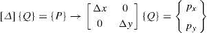 (25)
(25)
where sub-matrices [Δx],[Δy], are assembled with the known projection of the lengths for each direction in the plan, and {px},{py}, the column point load vector with particular values (in case of sole gravitational load), {px}={py}=0. The unknown diagonal density matrix , {Q }, is then easily obtained.
Some independent parameters, p , have to be determined a priori, obtaining density values for the other branches. The number of independent parameters, p , will correspond to the final value resulted from subtracting the rank of the matrix, [Δ], from the total number of branches, m:
 (26)
(26)
And for a half-quadrant configured with a cross rib , a tierceron and a side arch , only one valid solution exists, different to zero, {Q}={q1,q2,...,qm}≠{0}m, if the matrix system is resolved respecting the direction of the side arch , and in this case for the x axis.
 (27)
(27)
The augmented Row-echelon matrix , 〈[Δx] | [0] 〉, is singular , and therefore design is a parametric: rank〈[Δx] | [0] 〉 < n, det 〈[Δx] | [0] 〉=0. The number of parameters, p , depends on the rank of the sub-matrix, [Δx], because rank 〈[Δx] | [0] 〉 = rank [Δx]. Rank [Δx]=23, and branches are m=qm=26, so the total data-parameters may be p = 3.
For this particular example, the number of parameters does not change, regardless of the number of branches into which the ribs are subdivided by half-quadrants. Moreover, due to the geometrical independence of the ribs, a parameter may be defined for each one of the ribs , one for the cross rib , another for a tierceron and lastly for the side arch .
Once Force densities of all the branches have been obtained by Eq. (27), the vertical coordinate of the nodes is determined thanks to the basic equilibrium equation, {pz}=[Dz]{z}, depending on gravitational load.
The geometry is finally drawn with the value of the thrusts , Hx, Hy, on the supporting node of the vault, n a :
 (28)
(28)
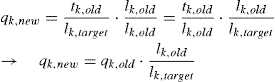
where [Δ]1 is the matrix of length projections for the branches next to the starting node, 1, {Q}1, corresponds to the column vector of densities and {H }, the column vector of the thrusts . Figure 18 shows two possible geometries in equilibrium, drawn by the three ribs in the whole side of the plan.

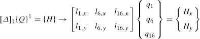
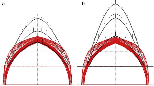
The next step may include the initial funicular inside the safety limits of the vault. The procedure will be to add the Numerical algorithm , N-FDM , to the Analytical method , A-FDM , thanks to which it will be possible to draw the sequential geometric approximations to the funicular by an iterative process (Fig. 19 b), changing the three independent parameters of the analytical basis little by little, e.g. both thrusts , H x, H y , and one density value (branch number 1), q 1 .
Fig. 19 A+N-FDM Astorga: minimum thrust line. (a) Initial funicular analysis, and (b) geometric adjustment.
The Force densities are recalculated in each new iteration, q m , as well as the lengths of each of the branches, l m , due to changing the nodes in the vertical direction. However, as can be seen in Figures 18 and 19, tridimensional funicular are not totally traced inside the safe thickness of the arch, flanked by the maximum and minimum thrust lines .
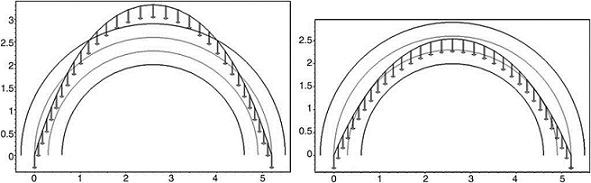
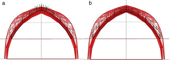
As a possible solution is to modify the height of the initial position of the start line, i.e. the new location of starting nodes is moved vertically. The value corresponds to the height, +2.1028 m (Fig. 20). This option involves reorganizing the original discretization of the ribs as a result of the recalculation of the point load, depending on the new attributed area, and it is the same for all nodes.
The guidelines may follow the Numerical method , N-FDM , as described above: (1) Obtain the initial geometry for both the maximum and minimum thrust lines (Fig. 20). (2) Adjust the three dimensional funicular of each rib, cross rib , tierceron and side arch using the numerical-iterative technique until they fit within the safety limits of the vault (Fig. 21).
3.3. Discussion
The Analytical method , A-FDM , is particularly suitable for known geometry, and it has been successfully developed into funicular analysis , to test the equilibrium of masonry structures.
The Numerical algorithm , N-FDM , can be used as a general design tool in structural analysis as a first stage of the overall process. Regularization of either the length or force of each element is considered a feasible means of optimization.
Although the theory has been only applied to gravitational loads (self-weight as vertical point load), N-FDM does not limit the direction of loads (two or three components can exist), and therefore this method is more general than the analytical one, and could be used when combining dead and wind load.
Lack of convergence would be controlled by reducing the number of constraints and repeating the iterative process until convergence occurs.
Recalculating the load, depending on the new attributed area for each new iteration, is tedious and complicated, and it could be of interest to use other automated methods of work in the future, such as plug-in Grasshopper ® .
Parametric control makes it possible to assign constraints to every element in a direct process that facilitates the checking of the resulting geometry.
4. Conclusions
Form-finding defines the design process for flexible structures as an independent stage prior to analysis and sizing, and it determines possible geometry based on a particular set of loads. Geometry here is therefore the unknown, which makes this process unusual. The solution to the problem need not be unique.
Form-finding means a procedure for seeking, evaluating and obtaining geometry.
The Force Density Method , FDM , is chosen for its many advantages over all other form-finding methods:
The Non-iterative method is used, at least to determine initial geometry.
A system of linear equilibrium equations is applied.
There is no need for pre-sizing: the equilibrium equations are linearized by assuming the relationship between the forces in the bars and their lengths as data, called Force density , q k , for the branch k , which also means there is no pre-sizing of the elements.
Equations are uncoupled for the three coordinates, x , y , z . Working independently using coordinates and assigning individuals constraints.
There are no restrictions on topology regarding the projection of lengths: Geometry is not fixed in the plan.
No single orthogonal discretization of the mesh is indispensable, as another one could be used.
Geometry is not limited to constant values of thrust (projection of forces).
The original FDM has been extended by successive contributions to its nomenclature and application. The method has been used not only for tensile structures , but has also been used for masonry, surfaces and the design of structures with tension and compression, as tensegrities .
This paper proposes two new algorithms that are useful as a general tool in structural design: Analytical method , A-FDM , and Numerical method , N-FDM , implemented through the application of: (1) Assembly of an unconstrained Connectivity matrix , [Du], (2) Combination of matrix and indicial notation in linear equilibrium equations, and (3) Mathematical software with symbolic capability (Maple ®).
The Analytical method , A-FDM , allows rewriting of the equilibrium equations in terms of other variables, such as projection of lengths or thrust.
The Numerical algorithm , N-FDM , enables optimization through an iterative process by regularizing the lengths towards a target , ltarget. The target value does not need to be unique, and it could be multiple based on a pre-defined design. Two new algorithms have been applied to funicular analysis: the evaluation of a known geometry and verification of a safe design for masonry .

