


 text new page (beta)
 English (pdf)
 Article in xml format
 Article references
 Send this article by e-mail
 Cited by SciELO
  Similars in
SciELO
Similars in
SciELO 
 Permalink
1. Introduction
Price predictability of a particular security is at the core of the activities of thousands of workers in the financial industry. From an academic standpoint, whether asset prices can be predicted using historical information relates to the evolution of the Efficient Market Hypothesis (EMH). In his seminal work, Fama (1970) describes an efficient market as one in which prices incorporate new information quickly and rationally. The EMH implies that if a market were to be efficient, prices will reflect all past and present information and any newly acquired information would be incorporated into the price instantaneously. If this hypothesis holds, then prices would follow a random walk and it would not be possible to generate and earn excess profits systematically (Malkiel, 2003). Simply put, as all the information is already incorporated into the price, the EMH implies that due to the stochastic behavior of prices, they cannot be predicted using past or present data.
Building over this hypothesis, the process of price forecasting typically assumes, not without an observational support, that markets are not efficient, therefore a price structure to be predicted can be expected. As stated by Hayek (1945), a price system plays a crucial role in incorporating information, the more relevance of such information, the greater the benefit that one agent can obtain in comparison to others. Under this perspective, it is common to find studies exploring the predictive possibility using daily, weekly or monthly returns. However, with the increasing availability of tools that allow the management and analysis of higher frequency data, new contributions can be made to the EMH’s framework.
Violations to the EMH are known as anomalies, a term introduced by Ball (1978), and have been thoroughly discussed, both with high and low frequency data. Hendershott and Riordan (2011) argue that financial instrument prices have non-stationary and non-linear behavior due to the variety of agents operating in a given market, each with a different investment horizon and objective and covering the range from long term investors to intraday speculators to algorithms operating from a server in a datacenter. All agents affect the market not only individually but from their collective actions. The result of this interaction is encoded in a single price signal. Cohen et al. (2002) state that large investors contribute to the efficiency of markets by, first, accelerating the incorporation of information in prices and, second, by offsetting the irrational behavior of individual investors.
However, there are studies that argue that a diversity in participants in the market, with different positions, strategies, points of view and behaviors, creates a signal with noise, resulting in a price signal with very complex behavior (Black, 1986; Jefferies et al., 2001; Giardina and Bouchard, 2003). One argument for this complex behavior is that the EMH does not account for network latency. Latency is the delay between a signal and a response, which is crucial for price formation, and when market participants have different latencies they will receive the same information at a slight time offset, and even if they all shared the same strategy, they would commit transactions asynchronously (Kirilenko and Lamacie, 2015).
It becomes clear that there is a need to develop modeling tools capable of incorporating non-linear elements that, by construction, can capture the complexity of the price generating process.
Some of the most common stock price forecasting methods include ARIMA, GARCH, Ordinary Least Squares, and Maximum Likelihood, all of which have been widely studied (Ariyo et al, 2014). However, building on the price forecasting literature that deals with complex signals, large amounts of high frequency data, and non-linear relationships in data, in the present work we propose the use of tools from the fields of Digital Signal Processing and Machine Learning as an attempt to outperform the traditional models when dealing with non-linear behavior of asset prices.
The proposed methodology consists of 2 steps. The first one involves the decomposition of the log-returns signal into simpler components based on methods in the field of Digital Signal Processing (DSP). These methods are commonly used for audio, image, and video processing, as well as data compression in order to decompose a complex signal into more manageable and simpler signals. In the context of financial price time series, the Wavelet transform has been used to split the single price signal with all its inherent complexity into several time series, each representing the behavior of the original signal across different frequency bands (Reboredo and Rivera-Castro, 2013; Chang and Fang, 2008; Caetano and Yoneyama, 2007). The expected result of this step is that by using wavelets to break up one time series into several time series (divided by frequency) and feeding them as inputs to the neural network model, the neural network will more easily learn how to use the short- and long-term information within the original signal. Due to the properties of the wavelet transform, all information in the original signal is retained in its wavelet representation.
After the wavelet transform, the second step consists of stacking a neural network. It is a Machine Learning technique that is able to capture the non-linear behavior contained in the prices. This Neurowavelet model has been used on traffic forecasting (Dunne and Ghosh, 2013), in streamflow forecasting (Mehr et al., 2013; Kisi, 2008), solar wind prediction (Nappoli et al., 2010). In financial time series analysis, the Neurowavelet model has been found to have superior performance to ARIMA and ARIMAX (Ortega and Khashanah, 2014). Building on the work of Ortega and Khashanah (2014), the novelty of this work lies in the use of a Maximal Overlap Discrete Wavelet Transform (MODWT) decomposition and a Long-Short Term Memory neural network and to predict the next period-return for frequencies of 1, 5 and 15 minutes.
The empirical strategy consists of using the information of the 25 most liquid assets in the Mexican Stock Exchange to perform their next-step prediction and compare the results with two alternative tools. The benchmark for this Wavelet-LSTM model is a Wavelet-Dense model, which uses a typical dense hidden layer instead of the LSTM hidden layer. Additionally, a conventional ARIMA (Box and Jenkins, 1970) model is also considered.
Our findings show that the Wavelet-LSTM outperforms, on average, both models. The remainder of the paper is structured as follows. The next section presents the literature review on wavelets, neural networks, and neuro-wavelets in finance. An explanation of the methodological aspects of the proposed model is found in the third section, followed by the description of data and the results of the empirical strategy. Concluding remarks are found in the last section.
2. Literature Review
2.1 Wavelets
Just as Ramsey (1999) stated, the contribution of wavelets to the finance field had great potential. By that time, several contributions had already been made, which can be reviewed in his work. Other noteworthy contributions are the work of Dremin and Leonidov (2008) where they filtered stock prices with a wavelet transform and found that the filtered series is characterized by volatility autocorrelation with large amplitude.
Caetano and Yoneyama (2007) use a wavelet decomposition to explain abrupt changes in stock prices while Aktan et al. (2009) propose the use of wavelets for the estimation of systematic risk in the Istanbul stock exchange, and Bruzda (2019) proposed their use to measure macroeconomic risk.
Building on their findings, we use a particular type of wavelet, the MODWT. This wavelet has been used to study asset prices because, as described by Zhu et al. (2014), it is useful to transform non-stationary and long-range dependent data into stationary and short-range dependent. On that end, Ardila and Sornette (2016) use the MODWT to analyze financial cycles. Ismail et al. (2016) compare a MODWT-EGARCH and a MODWT-GARCH model for prediction in African stocks, while Gupta et al. (2018) use a MODWT-VAR model to review the relationship between returns and volume in stock markets in India and China. Applications of MODWT for the Mexican or Latin-American case are, at most, scarce.
2.2 Neural networks
Neural networks are a Machine Learning tool used primarily for regression or classification tasks to approximate a function. They have also been used extensively in the study of financial data. However, some of the most notable works related to their performance in price forecasting, to our knowledge, are the ones by Maciel and Ballini (2008), Khashei and Bijari (2010), Adnan et al. (2011), Maknickiene and Maknickas (2012), and Ariyo et al. (2014), who found that a simple neural network outperforms SARIMA and GARCH models as well as other simple forecasting methods.
The type of neural network that seems to be a better fit for financial time series, particularly when modeling prices, is the recurrent neural network (RNN) due to its theoretical ability to retain information across time steps, Oancea and Ciucu (2014).
A problem that arises in practice is the difficulty for the RNN to reliably remember information from past time steps due to a phenomenon known as the Vanishing Gradient (Pascanu et al, 2013). Long-Short-Term-Memory (LSTM) is a type of RNN with gates that prevent the gradient from vanishing or exploding. LSTM introduces the concept of self-loops with context-conditioned weights. With a gated self-loop the time scale can be changed dynamically based on the input sequence. LSTM networks have been very successful in handwriting recognition, speech recognition, machine translation, and image captioning.
To that end, Fisher and Krauss (2018) state that LSTM is a suitable model for application in finance, although not much has been done. They find the LSTM outperforms a random forest, a deep neural net, and a logistic regression classifier when predicting the direction of change in the S&P500 index.
In a similar vein, Siami-Namini and Namini (2018) compare a LSTM neural network to ARIMA for the forecasting of financial data and find that former outperforms the latter. Choi and Lee (2018) use a series of stacked LSTM networks to predict financial time series and conclude that the model can capture non-linear behavior, while Hanson (2017) uses a LSTM neural network to forecast stock indices and shows that the outputs of the LSTM networks are similar to those obtained by ARMA and GARCH, but the neural network outperforms when predicting the direction of change.
2.3 Neurowavelets
Aussem and Murtag (1997) made one of the first works applying a wavelet decomposition and a neural network, they used a dynamic recurrent neural network trained on each resolution scale with the temporal-recurrent backpropagation algorithm and tested it on sunspots time series data.
The present work does not follow the neuro-wavelet concept introduced by Murtagh et al (2004), who define a wavelet network as a neural network in which activation functions have been replaced by wavelet functions. Instead, what we take a stance by using the concept of a neurowavelet as a layered model using first a wavelet transform, and then a neural network.
Such a model has been used in the prediction of financial time series by Minu et al. (2010), who find that a neurowavelet model outperforms GARCH and simple feedforward neural network models (FFNN models), while Zhang et al. (2001) used neurowavelet and FFNN models to forecast futures contracts and passed the forecast to a money management system to generate trades. They found that the neurowavelet model doubled the profit per trade.
More recently, Jamazi and Aloui (2012) use a wavelet and a multilayer backpropagation neural network to predict oil prices, they find the model performs better than the backpropagation neural network. Bao et al. (2017) use a wavelet transform followed by stack autoencoders and then a LSTM neural network for the forecast of the next day closing price for six market indices and their futures. They find their model outperforms a recurring neural network.
On the realm of high frequency data, Ortega and Khashanah (2014) apply a neurowavelet approach to 1-minute frequency data of Apple AAPL stock prices. They apply a non-decimated Haar wavelet decomposition followed by the Jordan (1997) and Elman (1990) networks, due to their ability to capture temporal patterns. They compare one, three and five-step ahead forecasting to ARIMA and ARIMAX and find that the neurowavelet model outperforms the other models. Arevalo et al. (2018) propose a discrete wavelet transform (DWT) and a deep neural network (DNN) to forecast one-minute and 3-minute log-returns of 19 stocks in the Dow Jones Index, and they find that the model has an accuracy rate between 64% and 76%. Our work is directly inspired by both studies and builds on them by proposing a neurowavelet model that uses Long Short-Term Memory (LSTM) units, which have internal logical gates that provide the model with an increased ability to remember data from previous time steps and to model even more complex non-linear behavior.
To the best of our knowledge, there is no existing literature that combines the Wavelet transform with an LSTM neural network in the context of high frequency price data.
3. Methodology
3.1 Wavelets and Neurowavelets
The proposed methodology consists of 2 steps. The first one involves the decomposition of the log-returns signal into simpler components using a MODWT transform, while the second one consists in stacking a neural network, commonly known as Neurowavelet.
Wavelets are an extension of Fourier analysis used to analyze nonstationary signals. According to Otazu (2008), the most important difference is that the Wavelet transform is defined in both the spatial frequency and spatial location, while the Fourier transform is only defined in spatial frequency. The Maximal Overlap Discrete Wavelet Transform (MODWT) is appropriate in the price forecasting process as it is time invariant (Percival and Walden, 2000).
Given the discrete wavelet transform with wavelet filter
On the other hand, neural networks are Machine Learning tools used primarily for regression or classification tasks to approximate a function
The basic elements of a neuron are: i) the connections between neurons -each carrying a weight that can be positive or negative-, ii) an adder -to sum the weighted input signals-; and iii) an activation function -to limit the amplitude of the output of a neuron in a linear or nonlinear manner-. The neuron can then be defined as shown in equations 3 and 4:
Where,
Unsupervised learning algorithms attempt to learn a structure within a dataset without explicitly linking an input state with an output state. The learning algorithm used here falls strictly under supervised learning. It is necessary to have a training set with a number of inputs that correspond to known outputs -target response-. The network is presented with a training example and the network weights are adjusted in order to minimize the error or the distance between the predicted response and the expected response.
In a neural network, neurons can be stacked layer upon layer, where every layer feeds its output as the input to the next layer. The output is directed, so there are no feedback connections, thus there is no recurrence. A feedforward neural network (FFNN) is defined as described by equation 5.
Where
The layers between the input layer and the output layer are known as hidden layers. By adding more hidden layers, the network can extract higher order statistics. Hidden layers are usually vectors, and their dimensionality determines the width of the model. Each element of the vector represents a neuron. This representation allows neurons to work as parallel units.
Neural networks are referred to in the form
Recurrent neural networks (RNN) are best suited to process sequential data
Recurrent nueral networks can scale to longer sequences than other types of networks. In that sense, the RNN updates the equations 6, 7 and 8 for every timestep between
Where
A problem that arises in RNN is that long term dependencies are not properly captured by the model because the gradients over timesteps either vanish or explode, resulting in instability during optimization (Pascanu et al., 2013). The exponentially smaller weights of long-term interactions eventually become so small that they lose effect. A widely used optimization algorithm to minimize the loss function during neural network training is stochastic gradient descent (Sirigiano and Spiliopoulos, 2017). This is the algorithm used in the empirical strategy of this work.
Because the computational cost of additive cost functions is
And it follows the estimated gradient in equation 10:
Where
However, in practice the learning rate is not fixed, it decreases gradually over time, so that the learning rate at iteration
As pointed out by Goodfellow et al., (2016), linear decay of the learning rate is often used in practice, which has the structure specified in equation 13:
Where
3.2 Long Short-Term Memory (LSTM) neurowavelets
Finally, the LSTM is a type of RNN with gates that prevent the gradient from vanishing or exploding (Hochreiter and Schmidhuber, 1997). LSTM introduces the concept of self-loops with context-conditioned weights.
With a gated self-loop, the time scale can be changed dynamically based on the input sequence. Each unit is composed of LSTM cells, and each cell has the same inputs and outputs as a common recurrent network, with more parameters and a system of gates for flow control. Let
Where
And the output gate
Where the internal state
3.3 Activation Function and Architecture
To get the output from one layer to the next in the neural network, an activation function is used. There is a wide variety of them and Gomes et al (2011) present a comprehensive review of activation functions in finance.
For the present work, the selected activation function is the sigmoid, which is described in equation 19, and which has an
The structure of the network determines how many neurons it has, the connections between them, and how the layers are stacked. The stacking of layers is what gives depth to the model.
The first layer can then be defined as shown in equation 20,
The second layer is shown in equation 21,
And layer
The universal approximation theorem (Hornik et al, 1989; Cybenko 1989) states that a feedforward network with a linear output layer and one or more hidden layers with any activation function can approximate any Borel measurable function from one finite-dimensional space to another with any desired non-zero error if the network has enough hidden units.
The derivatives of the feedforward network can also approximate the derivatives of the function. Any continuous function on a closed and bounded subset of
3.4 Optimization and Backpropagation
Optimization in neural networks consists of finding the parameters
Where
To minimize the objective function, the expectation is taken from the data generating distribution
In order to transform a machine learning problem into an optimization problem we minimize the expected loss on the training set by replacing the true distribution
A word of caution must be made regarding this approach as the empirical risk minimization can lead to overfitting - a situation where the model memorizes the training set and cannot be generalized properly for samples outside the training set.
Finally, backpropagation is the method used to allow a neural network to learn by itself. If a neuron
Where
The backpropagation algorithm applies a correction
Where
4. Data and Results
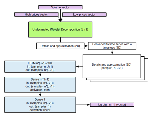
Figure 1 depicts the proposed methodology. The target output of our forecast is the log-return for one timestep in the future. Therefore, the two steps involved are:
Apply a MODWT to decompose the signal of log-returns.
Fit a LSTM neural network to the filtered data. The optimization target is the Mean squared error (MSE).
While this seems enough to build and train a Wavelet-LSTM neural network, in practice there are many hyperparameters inherent to the network that must be specified and their values can be the difference between the model converging or not converging, the speed of convergence, can result in overfitting, reaching different local minima, and computational cost.
The benchmark against which we compare the wavelet-LSTM model is an ARIMA model fitted to the data. We also compare the results to a wavelet-dense model in order to have a sense of the performance of the neural network itself.
We measure the ability of the model to reduce its mean squared error during training and to correctly forecast the direction -if the predicted return will be positive or negative-.
4.1 Data
We use price data from 25 assets of the Mexican Stock market with time intervals for 1, 5, and 15 minutes. The selection of assets is based on the largest market capitalization value of the Mexican Stock Exchange for the period of analysis. The selection of intervals is based on the availability of data from the data provider (Bloomberg), and on previous studies: Bakhach et al (2018) and Ortega and Khashanah (2014) make use of a 1 minute interval, Carrion (2013) uses a 5 minutes interval, Martens (2002) uses 5 and 15 minutes intervals. For internal validation purposes, the period of analysis goes from February 2017 to July 2017, considering the Open, Maximum, Minimum and Close prices, as well as Volume. Data were obtained from Bloomberg. The list of assets can be found in Table 1.
Table 1 List of assets from the Mexican Stock Exchange
| AMXL MM Equity | ELEKTRA* MMM Equity |
| WALMEX* MM Equity | PE&ONES* MM Equity |
| FEMSAUBD MM Equity | GCARSOA1 MM Equity |
| GFMEXICOB MM Equity | IENOVA* MM Equity |
| GFNORTEO MM Equity | ALFAA MM Equity |
| KOFL MM Equity | CUERVO* MM Equity |
| TLEVICPO MM Equity | KIMBERA MM Equity |
| SANMEXB MM Equity | GAPB MM Equity |
| CEMEXCPO MM Equity | ASURB MM Equity |
| AC*MM Equity | GRUMAB MM Equity |
| BIMBOA MM Equity | MEXCHEM* MM Equity |
| GFINBURO MM Equity | PINFRA* MM Equity |
Source: Own elaboration with tickers from Bloomberg (2017).
Both the Wavelet-LSTM and Wavelet-Dense models were initialized with a diverse combination of hyperparameters to determine convergence, stability, and performance. Then a training and calibration of 1926 experiments, each with a different combination of hyperparameters, was performed.
This requires considerable computing power, and for this we have assembled a small 8-node cluster with 12 Graphic Processing Unit, GPU, accelerator cards. To program and train the neural networks we use the Keras Deep Learning Library (version 1.0.4, Jun 06 2016) -an open source project started by Google researcher: Francois Chollet-.
The closing prices, C, are transformed to log returns and used as inputs for the benchmark ARIMA model. These log returns are also the output values and training target in the Wavelet-LSTM and Wavelet-Dense models.
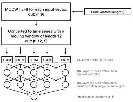
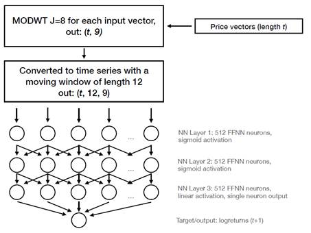
The time series for the 25 assets are separated in eight frequency levels using a MODWT transform with J=8. This decomposition generates 9 time series for each one of the 25 stocks analyzed, 8 detail series and 1 wavelet approximation. These time series are then divided into a moving window of size 12 and fed as input to a layer of 512 LSTM units, followed by a Dense layer fully connected with 512 neurons. It is finally followed by an additional Dense layer with 512 inputs and 1 output with a linear activation function, which corresponds to the forecast of the log returns. The Wavelet-LSTM and Wavelet-Dense models are illustrated in Figure 2 and Figure 3, respectively.
The time series are split 90% for training the network (training set) and 10% for out of sample validation (validation set). We trained the model with 500 epoch iterations (an epoch is one complete pass over the training data set), checking for congruence between the training error and validation error to avoid overfitting and detecting instability.
The optimization target used is the Mean Squared Error (MSE) and the scale is adjusted in the interval [-1,1] in order to match the original center to 0 so the sign of the return can be preserved while pairing the interval to the one of the activation functions.
Finally, to compare the performance of the Wavelet-LSTM model with the selected benchmarks, we count the number of times the sign of the forecast corresponds with the actual sign of the return, that is, the times the direction of the forecast is correct.
4.2 Results
When building a forecasting model, parsimony is desirable. A reduced number of estimated parameters is easier to understand and explain, and every estimated parameter adds estimation variation. In the case of ARIMA each unnecessary parameter causes the variance of the one step ahead forecast error to increase approximately, where
By finding a balance between goodness of fit and model complexity we can avoid overfitting. In the case of Machine Learning and more specifically the Wavelet-LSTM model proposed, we use a training set and an out-of-training-sample validation set, and we evaluate the loss function for each. If the training loss becomes measurably lower than the validation loss, we have a condition of overfitting or no convergence. One technique to prevent overfitting is Early Stopping, which halts the iterative training algorithm once the training loss compared to the validation loss shows no improvement. Table 2 contains the percentages of the correct direction predicted by ARIMA, Wavelet-LSTM y Wavelet-Dense models for each of the 25 stocks and the time scales selected. Table 3 contains the percentage difference in the performance of Wavelet-LSTM model against the selected benchmarks.
It can be seen that, on average, Wavelet-LSTM improves the forecasting of the one-step ahead direction when compared to the Wavelet-Dense and the ARIMA models.
For the case of the first benchmark, the biggest difference between the Wavelet-LSTM precision and the Wavelet-Dense appears in the 5 minutes window.
For the case of the second benchmark, as the time window becomes larger, the Wavelet-LSTM forecasting improvement increases in magnitude compared to the forecasting of the ARIMA model. Altogether, the results are in line with the ones exposed in the literature review.
Table 2 Percentage of correct prediction of the one-step ahead direction
| Wavelet-LSTM | Wavelet-Dense | ARIMA | |||||||
|---|---|---|---|---|---|---|---|---|---|
| Stock | 1m | 5m | 15m | 1m | 5m | 15m | 1m | 5m | 15m |
| AMXL MM Equity | 25.74% | 37.34% | 46.80% | 25.90% | 36.40% | 49.97% | 25.51% | 36.20% | 42.55% |
| WALMEX* MM Equity | 36.59% | 45.44% | 51.89% | 36.30% | 42.68% | 50.88% | 35.16% | 42.84% | 45.77% |
| FEMSAUBD MM Equity | 41.39% | 48.69% | 54.46% | 41.21% | 47.91% | 50.93% | 42.23% | 47.46% | 49.66% |
| GFMEXICOB MM Equity | 36.62% | 46.16% | 52.88% | 36.18% | 44.36% | 48.17% | 34.84% | 43.39% | 46.78% |
| GFNORTEO MM Equity | 34.99% | 42.87% | 53.25% | 35.14% | 47.08% | 51.29% | 34.90% | 44.45% | 47.97% |
| KOFL MM Equity | 40.41% | 49.45% | 48.15% | 40.43% | 48.40% | 55.49% | 40.05% | 46.64% | 49.33% |
| TLEVICPO MM Equity | 42.46% | 54.74% | 57.34% | 41.31% | 48.35% | 52.70% | 40.97% | 46.31% | 47.90% |
| SANMEXB MM Equity | 34.15% | 43.92% | 50.11% | 33.78% | 44.60% | 51.62% | 33.81% | 43.59% | 46.75% |
| CEMEXCPO MM Equity | 28.70% | 42.09% | 51.24% | 28.76% | 39.84% | 49.51% | 28.37% | 39.34% | 44.49% |
| AC*MM Equity | 38.32% | 49.47% | 53.94% | 38.04% | 47.76% | 51.75% | 37.63% | 46.23% | 48.33% |
| BIMBOA MM Equity | 32.15% | 48.17% | 52.95% | 31.37% | 41.97% | 51.34% | 31.09% | 40.91% | 46.43% |
| GFINBURO MM Equity | 33.33% | 58.21% | 68.86% | 30.23% | 42.61% | 49.31% | 29.66% | 39.96% | 45.64% |
| ELEKTRA* MMM Equity | 42.04% | 58.25% | 59.85% | 39.69% | 49.35% | 55.99% | 39.96% | 47.70% | 49.38% |
| PE&ONES* MM Equity | 40.79% | 52.54% | 59.10% | 40.04% | 47.54% | 56.90% | 39.28% | 46.89% | 48.89% |
| GCARSOA1 MM Equity | 35.79% | 46.27% | 53.19% | 34.10% | 43.64% | 54.87% | 34.20% | 41.92% | 46.63% |
| IENOVA* MM Equity | 34.61% | 50.91% | 57.03% | 34.20% | 45.24% | 52.93% | 32.13% | 40.12% | 44.43% |
| ALFAA MM Equity | 32.01% | 47.82% | 53.56% | 30.60% | 42.35% | 50.49% | 30.41% | 40.05% | 44.88% |
| CUERVO* MM Equity | 25.65% | 37.59% | 44.16% | 25.25% | 34.63% | 45.09% | 25.00% | 35.41% | 41.98% |
| KIMBERA MM Equity | 34.85% | 54.41% | 62.92% | 31.29% | 42.17% | 45.00% | 30.93% | 40.10% | 45.02% |
| GAPB MM Equity | 39.23% | 49.55% | 55.15% | 39.21% | 47.20% | 56.40% | 38.24% | 45.04% | 48.28% |
| FUNO11 MM Equity | 28.50% | 41.29% | 50.26% | 28.34% | 39.01% | 49.87% | 27.88% | 37.52% | 43.67% |
| ASURB MM Equity | 38.78% | 49.82% | 57.47% | 39.31% | 48.39% | 49.07% | 38.79% | 46.59% | 47.79% |
| GRUMAB MM Equity | 35.29% | 46.52% | 51.59% | 33.44% | 45.48% | 51.03% | 34.98% | 44.75% | 48.33% |
| MEXCHEM* MM Equity | 33.60% | 52.13% | 57.27% | 32.64% | 43.57% | 57.34% | 32.88% | 42.19% | 47.41% |
| PINFRA* MM Equity | 35.75% | 48.34% | 53.14% | 35.80% | 45.76% | 50.87% | 34.95% | 44.53% | 48.15% |
Source: Own elaboration with the results of the study.
Table 2 contains the percentages of the correct direction predicted by ARIMA, Wavelet-LSTM y Wavelet-Dense models for each of the 25 stocks and the time scales selected. It can be seen that, in general, the Wavelet-LSTM yields higher percentages of correct prediction than those from the Wavelet-Dense and the ARIMA models. Of the predictions considering a 1-minute window, the Wavelet-LSTM has the highest percentage in 18 out of the 25 forecasts. The average of correct prediction for this window is 35.27% for the Wavelet-LSTM, while for the Wavelet-Dense and the ARIMA models the average are 34.5% and 34.15% respectively. For the 15 minutes window, again, the Wavelet-LSTM has the highest percentage in 18 out of the 25 forecasts. Interestingly, the average of correct prediction increases for the three models: 54.26% for the Wavelet-LSTM, 51.55% for the Wavelet-Dense and 46.66% for the ARIMA model. Finally, for the 5 minutes window the Wavelet-LSTM has the highest percentage in 23 out of the 25 forecasts and the average of correct prediction is 48.08% for the Wavelet-LSTM, 44.25% for the Wavelet-Dense and 42.81% for the ARIMA model. In sum, the Wavelet-LSTM outperforms both benchmark models in 59 of the 75 forecasts and appears to be more precise in the 5 minutes window than the Wavelet-Dense and the ARIMA models.
Table 3 Difference of correct prediction between Wavelet-LSTM model and benchmarks
| Wavelet-LSTM | ARIMA | Wavelet-LSTM | Wavelet-Dense | |||||
|---|---|---|---|---|---|---|
| Stock | 1m | 5m | 15m | 1m | 5m | 15m |
| AMXL MM Equity | 0.22% | 1.14% | 4.25% | -0.16% | 0.94% | -3.17% |
| WALMEX* MM Equity | 1.43% | 2.60% | 6.12% | 0.29% | 2.76% | 1.01% |
| FEMSAUBD MM Equity | -0.84% | 1.23% | 4.80% | 0.17% | 0.78% | 3.53% |
| GFMEXICOB MM Equity | 1.78% | 2.77% | 6.10% | 0.44% | 1.79% | 4.71% |
| GFNORTEO MM Equity | 0.09% | -1.58% | 5.28% | -0.15% | -4.22% | 1.96% |
| KOFL MM Equity | 0.37% | 2.80% | -1.18% | -0.01% | 1.04% | -7.34% |
| TLEVICPO MM Equity | 1.49% | 8.44% | 9.45% | 1.14% | 6.39% | 4.65% |
| SANMEXB MM Equity | 0.34% | 0.33% | 3.36% | 0.37% | -0.67% | -1.51% |
| CEMEXCPO MM Equity | 0.33% | 2.75% | 6.75% | -0.06% | 2.25% | 1.73% |
| AC*MM Equity | 0.69% | 3.23% | 5.61% | 0.28% | 1.71% | 2.19% |
| BIMBOA MM Equity | 1.06% | 7.26% | 6.51% | 0.78% | 6.20% | 1.60% |
| GFINBURO MM Equity | 3.67% | 18.25% | 23.22% | 3.10% | 15.60% | 19.55% |
| ELEKTRA* MMM Equity | 2.08% | 10.55% | 10.47% | 2.35% | 8.91% | 3.86% |
| PE&ONES* MM Equity | 1.51% | 5.65% | 10.20% | 0.75% | 5.00% | 2.19% |
| GCARSOA1 MM Equity | 1.58% | 4.35% | 6.56% | 1.69% | 2.64% | -1.68% |
| IENOVA* MM Equity | 2.48% | 10.79% | 12.60% | 0.41% | 5.66% | 4.10% |
| ALFAA MM Equity | 1.60% | 7.77% | 8.68% | 1.40% | 5.47% | 3.07% |
| CUERVO* MM Equity | 0.65% | 2.18% | 2.18% | 0.41% | 2.97% | -0.93% |
| KIMBERA MM Equity | 3.93% | 14.32% | 17.90% | 3.56% | 12.25% | 17.92% |
| GAPB MM Equity | 1.00% | 4.51% | 6.87% | 0.02% | 2.35% | -1.24% |
| FUNO11 MM Equity | 0.62% | 3.77% | 6.59% | 0.16% | 2.27% | 0.39% |
| ASURB MM Equity | -0.02% | 3.23% | 9.69% | -0.54% | 1.44% | 8.41% |
| GRUMAB MM Equity | 0.31% | 1.77% | 3.26% | 1.84% | 1.04% | 0.56% |
| MEXCHEM* MM Equity | 0.73% | 9.94% | 9.86% | 0.96% | 8.56% | -0.07% |
| PINFRA* MM Equity | 0.81% | 3.81% | 4.99% | -0.05% | 2.57% | 2.27% |
| Average | 1.12% | 5.27% | 7.61% | 0.77% | 3.83% | 2.71% |
Source: Own elaboration with the results of the study.
Table 3 contains the percentage difference in the performance of Wavelet-LSTM against the selected benchmarks. For this analysis, if a positive sign is obtained, the Wavelet-LSTM yielded a higher percentage of correct prediction than the one from the Wavelet-Dense or the ARIMA models. For the case of the difference in percentage of correct prediction between the Wavelet-LSTM and the Wavelet-Dense, 60 out of the 75 forecasts showed a positive sign. This suggests that the Wavelet-LSTM outperformed the Wavelet-Dense in 80% of the presented forecasts. When analyzing the case of the difference in percentage of correct prediction between the Wavelet-LSTM and the ARIMA model, the positive sign is obtained in 71 of the 75 cases, for an outperformance of approximately 95% of the presented forecasts. Altogether, the results are in line with the ones exposed in the literature review: in general, the ARIMA model is outperformed by both Wavelet models, while the Wavelet-Dense is outperformed by the Wavelet-LSTM.
5. Concluding Remarks
The description of price dynamics at various frequencies is of importance both for academics and practitioners in finance. Many are particularly concerned with the possibility of forecasting prices or returns in a specific time horizon.
Previous studies have shown that at high frequencies, returns do not follow the efficient markets hypothesis, hence a “complete” stochastic behavior is not observed (Nath and Dalvi, 2004; Strawińsky and Slepaczuk, 2008; Tapia, 2020). By asset prices not following a random walk a forecasting of their next value is possible and, with the use of novel tools and computational power, one might take advantage of this fact. This directly translates to a potential benefit for the practitioners that have recognized the importance of dealing with high frequency information in their predictive models. Precisely, O’Hara (2014) discussed a new market paradigm: “Trading has become faster, and market structure has fundamentally changed. In today’s market, high-frequency traders (HFTs) act on information revealed by low-frequency traders (LFTs). To survive, LFTs must avoid being detected by predatory algorithms of HFTs. LFTs can thrive by adopting trading strategies appropriate to the high-frequency trading world”.
5.1 Main Results
In the present work, we apply a wavelet followed by LSTM neural network to 25 assets of the Mexican Stoc Market. We compare the performance of the proposed model with the performance of an ARIMA model and a wavelet followed by a Dense neural network model, following the literature.
The measure for comparison is the accuracy in forecasting the direction of the price movement (the sign of the logarithmic return) for time series at three different time windows (1, 5 and 15 minutes).
We find that The LSTM neuro-wavelet outperforms both the ARIMA and the Dense neuro-wavelet for the three studied frequencies. However, the higher accuracy was found for the 5 minutes interval.
5.2 Limitations and Recommendations for Future Research
Results and implementation do not come without limitations. We recognize that the selection of the benchmark models and high market capitalization assets may lead to skewed results. While we selected Wavelet-Dense and ARIMA models based on the consensus when dealing with financial time series, a comparison against other Neurowavelets architectures might be of interest.
On the other hand, we also find value in exploring the proposed methodology in various cases within the Mexican market, such as, considering different market capitalization levels or considering industry indices instead of single assets. We leave that for future research.
Finally, the technical capacity surely represents a constraint for the hyperparameters’ selection and estimation capability may be somewhat hindered by it. In that sense, future research agenda may also include the assessment of whether these results are maintained over long time windows or in markets with a different inherent structure, such as the US stock market.
5.3 Originality
The question of whether prices can be forecasted is not new, the literature on the topic is vast, but most of it focuses on low frequency operations. With the mass availability of computing power, large amounts of data and new filtering tools, we can revisit the question, and particularly, we can bound it to the realm of high frequency trading.
Wavelet filtering has been widely applied in finance. Neural network models have been extensively explored, as well. But recently, the application of both models combined has been proposed (Zhang et al., 2001; Minu et al., 2010; Jamazo and Aloui, 2012; Bao et al. 2017). For high frequency trading, little has been done. Ortega and Khashanah (2014) apply a Haar wavelet followed by a Jordan-Elman neural network to 1 minute data for the Apple (AAPL) stock price. Arevalo et al. (2018) apply a wavelet followed by a Deep Neural Network (DDM) to 1 and 3 minute data on 19 stocks in the Dow Jones Index.
We follow this line, by applying a wavelet transform followed by a Long Short Term Memory neural network, which provides increased ability to remember data from previous time steps, and thus allows to model more complex non-linear behavior.
5.4 Main Conclusions
In this work we illustrate the use of a new tool for forecasting stock prices at high frequencies. The results show that the LSTM neuro - wavelet model proposed outperforms the chosen benchmarks. This leads us to conclude that the addition of this tool to the forecasting toolkit of a market participant would be of great value. Certainly, the application of said tool is computationally intensive, but the possible gains from it, and the ever-greater availability of computing power might make it possible to consider the use of complex algorithms, such as this one.
We believe there is an opportunity to outperform traditional forecasting tools by making clever use of computer power, and such we have tried to show in the present research. This is an important step in showing how ever more sophisticated tools can be applied successfully to gain insight into the structure of the markets and the complexity that interactions of many actors induce.

