


 text new page (beta)
 English (pdf)
 Article in xml format
 Article references
 Send this article by e-mail
 Cited by SciELO
  Similars in
SciELO
Similars in
SciELO 
 Permalink
1. Introduction
Daniels (1951) describes: "Fashion is important because it is in almost everything." In modern times a fashion started in a metropolitan area in one country tends to rapidly globally spread over the world due to modern communications. Fashion has become a very important industry. According to Hemphill and Suk (2009: 1148), "It is the major output of a global business with annual U.S. sales of more than $200 billion - larger than those of books, movies, and music combined. (···). It has provided economic thought with a canonical example in theorizing about consumption and conformity. Social thinkers have long treated fashion as a window upon social class and social change. Cultural theorists have focused on fashion to reflect on symbolic meaning and social ideals." There are many studies about fashion and its interactions with other aspects of societies, even though the literature on formally modelling economics of fashion are not so many (e.g.,Pollak, 1976; Stigler and Becker, 1977; Abel, 1990; Karni and Schmeidler, 1990; Bianchi, 2002; Nakayama and Nakamura, 2004; Caulkins, et al., 2007; Zhou, et al., 2015). Simmel (1904) points out that fashion dynamics is enforced by common people's imitation of elite. Giovinazzo and Naimzada (2015) build a model to investigate the dynamics of the fashion cycle described by Simmel (1904). They argue that the originality of Simmel's thought has been lost in the modern literature on the subject. A main reason is that the... "models generally assume that preferences are exogenous and overlook the fact that individual tastes change in time, partly in line with choices previously made by the social group." Nevertheless, there are only a few formal economic models which explore dynamic complexity of fashion within context of economic growth and development theory. An analytical reason for this slow development is that how to deal with heterogeneity of goods and households with microeconomic foundation are still challenging issues in economics. The lacking of a proper analytical framework means that it is difficult for economists to deal with fashion and wealth accumulation in an integrated theory.
As far as fashion and classification of the population are concerned, this paper is inspirited by the economic model of fashion by Giovinazzo and Naimzada (2015). Their model is based on Benhabib and Day (1981). The population in their model is classed into the snob and the bandwagoner (Leibenstein, 1950). In their model there are one conspicuous good and one normal good. The bandwagoner's preference is characterized by that a particular kind of consumption increases in association with the rise in the social group's average consumption of the previous period. The snob's preference for a certain purchase falls with the rise of the average collective consumption of the preceding period. We use this idea to take account of fashionable behavior and their impact on macroeconomic as well as microeconomic variable in a general equilibrium dynamic model proposed by Zhang (2012, 2013). It should be remarked that Shi (1999) builds a wealth accumulation model with fashion and two groups of agents. Fashion is treated as an externality due to dependence of individual agents' time preference on the two groups' per-capita consumption habit. In Shi's approach stronger and more persistent fashion tends to generate oscillations in wealth. This study differs from Shi's approach in that Shi employs the traditional Ramsey approach to household behavior and this study uses Zhang's approach (Zhang, 1993, 2012). The paper is organized as follows. Section 2 develops the growth model of wealth and income distribution among heterogeneous households with fashion. Section 3 examines dynamic properties of the model and simulates the model with three groups. Section 4 carries out comparative dynamic analysis. Section 5 concludes the study.
2. The Basic Model
We consider an economic system consisting of fashion, capital goods, and consumer goods sectors. The capital goods and consumer goods sectors are the same as in the Uzawa two sector model (Uzawa, 1961; Burmeister and Dobell 1970; and Barro and Sala-i-Martin, 1995). Services are classified as consumer goods. The fashion sector produces fashion goods. It should be noted that it is straightforward to further classify fashion goods as durable and instantly consumed goods. For simplicity of analysis, we consider fashion goods as instantly consumed goods. Capital goods are be used as inputs in the three sectors. Capital depreciates at a constant exponential rate δk (0 < δk < 1) , which is independent of the manner of use. Households own assets of the economy and distribute their incomes to consume and save. Exchanges take place in perfectly competitive markets. Factor markets work well; factors are inelastically supplied and the available factors are fully utilized at every moment. Saving is undertaken only by households. All earnings of firms are distributed in the form of payments to factors of production, labor, managerial skill and capital ownership. Rather than classifying the population into the snob, the bandwagoner as in Giovinazzo and Naimzada (2015), we classify the population into the snob, the bandwagoner, and common consumer. The population consists of three groups, called consumers (who have no interest in fashion), the snob, and bandwagoner. Each group has a fixed population Ñj, indexed by j = C, S, B. Let prices be measured in terms of capital goods and the price of the commodity be unity. We denote the wage rates and rate of interest by wj(t) and r(t) respectively. Let pC(t) and pF(t) denote prices of consumer and fashion goods, respectively. The total capital stock K(t) is allocated between the three sectors. We use subscript index, i, s and f to stand for capital, consumer, and fashion goods sectors, respectively. We use Nm(t) and Km(t) to stand for the labor force and capital stocks employed by sector m. The total population Ñ and total qualified labor supply N are
in which hj is the human capital of group j. The assumption of labor force being fully employed implies
2.1 The Capital Goods Sector
Let Fm(t) stand for the production function of sector m, m = i, s, f. The production function of capital goods sector is specified as follows
where Ai, αi and βi are positive parameters. The marginal conditions for the capital goods sector are given by
where wt is the wage rate of per qualified labor input. It should be noted that the wage rate of group j is
2.2 Consumer Goods and Fashion Goods Sectors
The production functions of the two sectors are
where Am, αm and βm are the technological parameters of the two sectors. The marginal conditions are
2.3 Current Income and Disposable Income
In this study, we use the approach to modeling behavior of households by Zhang (1993). Let
The per capita disposable income is the sum of the current disposable income and the value of wealth. That is
2.4 Budget Constraints with Fashion Goods
The disposable income is used for saving and consumption. The representative household from group j would distribute the total available budget between savings sj(t) consumer goods cj(t) and fashion goods fj(t). It should be noted fC(t) = 0. As far as no confusion occurs, we similarly use indexes without explicitly distinguishing groups. The budget constraints are
2.5 Utility Functions with Fashion
We assume that utility level Uj(t) is dependent on cj(t), sj(t) and fj(t) as follows
where ξj0(t), is the propensity to consume consumer goods, λj0(t) the propensity to save, and θj0(t) is group j's propensity to consume fashion goods (remark, θC0(t) = 0). Following Giovinazzo and Naimzada (2015), we consider the propensities of the snobs and the bandwagoners for consuming fashions endogenous. We will specify preference changes later on. It should be noted that although there are many heterogeneous-households growth models with endogenous wealth accumulation, the heterogeneity in most of those studies is by the differences in the initial endowments of wealth among different types of households rather than in preferences (see, for instance, Chatterjee, 1994; Caselli and Ventura, 2000; Maliar and Maliar, 2001; Penalosa and Turnovsky, 2006; and Turnovsky and Penalosa, 2006). Different households are essentially homogeneous in the sense that all the households have the same preference utility function in the approach.
2.6 Optimal Household Behavior
Maximizing the utility function subject to (9) yields
where
2.7 A Simplified Literature Review on Fashion Dynamics and Habit Formation
Before we specify how θS0(t) and θB0(t) change over time, we review the approach to fashion in discrete time accepted by Giovinazzo and Naimzada (2015). Their model is based on Benhabib and Day (1981). The population is classed into the snob and the bandwagoner, subscripted by i = SB. There are one conspicuous good and one normal good. The bandwagoner's preference is characterized by that a particular kind of consumption increases in association with the rise in the social group's average consumption of the previous period. The snob's preference for a certain purchase falls with the rise of the average collective consumption of the preceding period. The utility function is specified as
where xi and yi are respectively the consumption levels of conspicuous good and normal good by i. The budgets with constant prices are
It should be noted that price is fixed in the approach. As the model is partial (and for short-term problems), the fixed prices assumption is acceptable. The population is normalized unity. The population shares of the bandwagoners and the snobs are respectively w and 1 - w. The average conspicuous consumption of period t is
The snob's preference change is given by
where
Each individual takes the average behavior of large populations
We also generally assume that θS(t)
θB(t)) is decreasing
(increasing) in
2.8 Wealth Accumulation
According to the definition of sj(t) the change in the household's wealth is given by
This equation states that the change in wealth is equal to saving minus dissaving.
2.9 Demand and Supply of the Three Sectors
The demand and supply equilibrium for the consumer goods sector is
The demand and supply equilibrium for the fashion sector is
As output of the capital goods sector is equal to the depreciation of capital stock and the net savings, we have
where
2.10 Capital being Fully Utilized
Total capital stock K(t) is allocated to the three sectors
We completed the model. The model is structurally general in the sense that some well-known models in economics can be considered as its special cases. For instance, if the population is homogeneous and there is no fashion industry, our model is structurally similar to the neoclassical growth model by Solow (1956) and Uzawa (1961). It is structurally similar to the Walrasian general equilibrium model (note that in our approach the population can be classified into any number of groups) if the wealth is fixed and depreciation is neglected. The new aspect of this paper is the introduction of fashion into the general equilibrium growth model proposed by Zhang.
3. The Dynamics and its Properties
As the dynamic system is nonlinear and highly dimensional with wealth accumulation, it is difficult to get explicitly analytical properties. We can conduct simulation to follow the motion of the dynamic system. The following lemma shows that the dimension of the dynamical system is the same as the number of groups. We also provide a computational procedure for calculating all the variables at any point in time. First, we introduce a new variable z(t).
3.1 Lemma
The motion of the economic system is determined by differential equations with
z(t),
in which
The lemma gives a computational procedure for following the motion of the economic system. We specify the preference changes as follows
where
where wB and wS are "weight" parameters. For instance, if wB is small, it simply implies that a change in the propensity to consume fashion is associated with a relatively small change in the propensity to consume consumer goods and a relatively large change in the propensity to save. Under (24) and (25) we have
We have that ρj(t) are constant. From (11) and (10) we have
where we use (26). Inserting (24) in (27) yields.
We specify parameter values as follows
The population of the consumer is largest, while the population of the bandwagoner is the next. The capital goods and consumer goods sector's total productivities are respectively 1.3 and 1. We specify the values of the parameters, αj in the Cobb-Douglas productions for the capital goods and consumer goods sectors approximately equal to 0.3 (for instance, Miles and Scott, 2005; Abel et al., 2007). The depreciation rate of physical capital is specified at 0.05. A change in the propensity to consume fashion is associated with the equal changes (in the opposite direction) in the propensities to consume and to save. We specify the initial conditions as follows
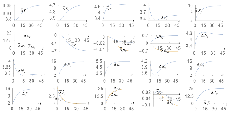
The motion of the variables is plotted in Figure 1. In Figure 1, the national income is
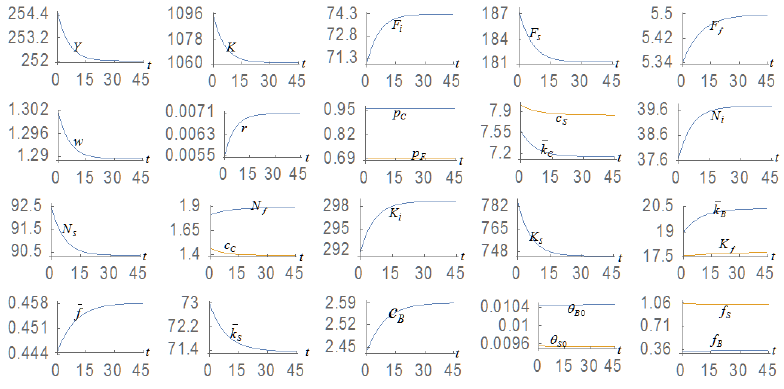
Due to the fixed positions of the initial state, the national output and wealth/capital fall over time. The output level of the capital goods sector and fashion sector rise and the output level of the consumer goods sector fall overtime. The price of consumer goods falls. The rate of interest rises in association with falling wage rates. The prices of consumer goods and fashion goods and the propensities to consume fashion goods change slightly. Labor force is shifted from the consumer goods sector to the other two sectors. The capital input of the consumer goods sector is reduced and the capital inputs of the two other sectors are increased. The snob consume slightly less fashion goods and the bandwagoner more fashion goods. The average consumption level of fashion goods is increased over time. The snob consumes less consumer goods and has less wealth. The bandwagoner consumes more consumer goods and has more wealth. The consumer consumes less consumer goods and has less wealth.
Figure 1 shows that that all the variables become stationary in the long term. This implies the existence of an equilibrium point. The simulation confirms that the system has a unique equilibrium. We list the equilibrium values in (25)
It is straightforward to calculate the three eigenvalues as follows
The eigenvalues are real and negative. The unique equilibrium is locally stable. This guarantees the validity of exercising comparative dynamic analysis.
4. Comparative Dynamic Analysis
We simulated the motion of the national economy under (29). It is significant to examine how
the economic system reacts to exogenous changes. As the lemma provides the
computational procedure to calibrate the motion of all the variables, it is
straightforward to examine effects of change in any parameter on transitory
processes as well stationary states of all the variables. We introduce a variable
xj(t) which stands for the
change rate of the variable,
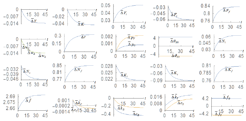
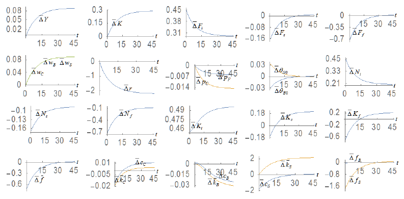
4.1 The Bandwagoner's Propensity to Consume Fashion Goods Being More strongly affected by the average fashion consumption
We now examine the effects that the bandwagoner's propensity to consume fashion goods is more strongly affected by the average fashion consumption as follows:
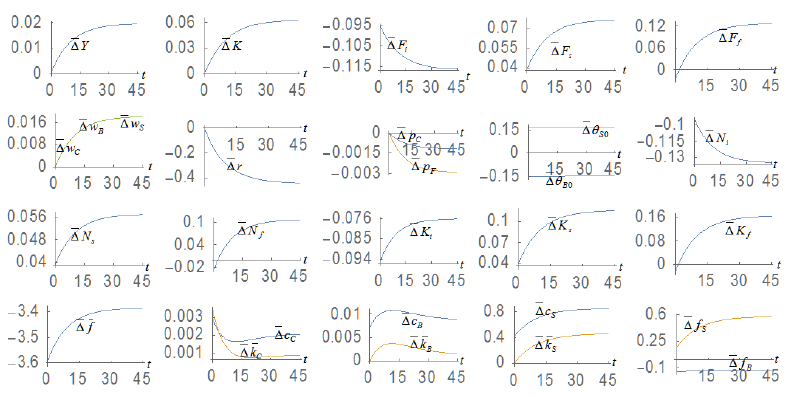
4.2 The Snob's Propensity to Consume Fashion Goods being More Negatively affected by the Average Fashion Consumption
We now examine the effects that the snob's propensity to consume fashion goods is more negatively affected by the average fashion consumption as follows:
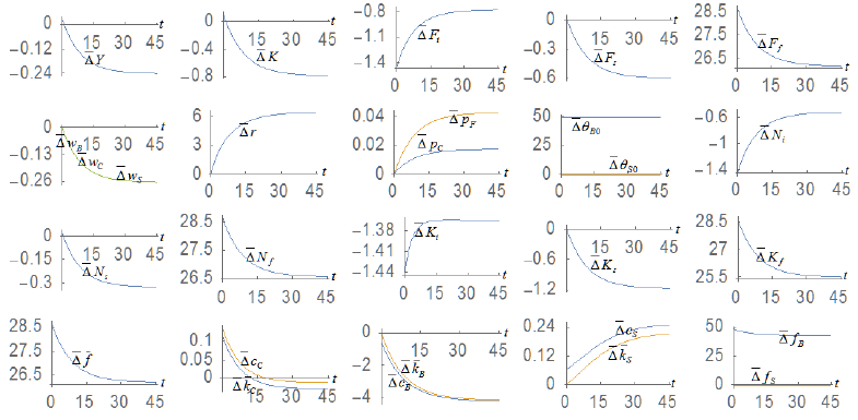
4.3 The Bandwagoner's Propensity to Consume Fashion Goods Being Increased
We now examine the effects that the intercept in the function of the bandwagoner's propensity to consume fashion goods is increased as follows:
4.4 The Bandwagoner's Human Capital Being Improved
We now examine the effects that the bandwagoner's human capital is improved as follows: hB: 2 ⇒ 2.5 The total labor is augmented. Each sector employs more labor force. The national wealth and output are increased. All the three sectors' output levels and capital inputs are augmented. The bandwagoner's wage rate is increased and the other two groups' wage rates are slightly affected. The rate of interest and prices of the consumer and fashion goods are reduced. The bandwagoner's preference to consume fashion goods is increased and the snob's preference to consume fashion goods is reduced. The average consumption of fashion goods is expanded. The bandwagoner consume more fashion and consumer goods and have more wealth. The snob consume less fashion goods. The snob consume more consumer goods and have more wealth initially and consume less consumer goods and have less wealth in the long term. The consumer's behavior is slightly affected in the long term.
4.5 A Rise in the Bandwagoner's Population
We now examine the effects that the bandwagoner's population is expanded as follows: NB: 10 ⇒ 11 The total labor is augmented. Each sector employs more labor force. The national wealth and output are increased. All the three sectors' output levels and capital inputs are augmented. All the wage rates are enhanced. The rate of interest and prices of the consumer and fashion goods are reduced. The average consumption of fashion goods is expanded. The bandwagoner's preference to consume fashion goods is lowered and the snob's preference to consume fashion goods is enhanced. The bandwagoner consume more fashion and consumer goods and have more wealth. The snob consume less fashion goods. The snob consume more consumer goods and have more wealth initially and consume less consumer goods and have less wealth in the long term. The consumer's behavior is slightly affected in the long term.

4.6 A Rise in the Snob's Propensity to Save
We now examine the effects that the intercept of the function of the snob's propensity to save as follows:
5. Concluding Remarks
This study dealt with interactions between fashion, economic growth and income and wealth distribution in an economic growth model of heterogeneous households with economic structure. The model emphasized the role of fashion on economic structural change and wealth and income distribution. It was inspirited by some ideas in the literature of economics of fashion. The model was developed within the framework of the integrated Walrasian general equilibrium and neoclassical growth theory by Zhang (2012, 2013). For illustration, we simulated the motion of the economic system. We identified the existence of a unique stable equilibrium point. We also carry out comparative dynamic analysis with regard to the snob's propensity to consume fashion goods, the bandwagoner's propensity to consume fashion goods, the bandwagoner's human capital, the bandwagoner's population, and the snob's propensity to save. We examined how changes in these parameters affect fashion development, wealth accumulation, and inequalities in income and wealth. From our simulation, we see that relations between fashion dynamics, inequality and economic growth are complicated in the sense that these relations are determined by interrelated in a very complicated manner. As our analytical framework is quite general, it is possible to generalize and extend the model in different aspects. One important direction is to introduce taxation into the general dynamic equilibrium model with fashion. We dealt with a simplified fashion dynamics. Fashion appears in arts, sciences, politics, academics, business, food, clothing, morality and entertainment in different forms and changes in different speeds. To analyze detailed structural changes within fashion industry in a macroeconomic framework with endogenous knowledge and wealth is a challenging issue in theoretical economics.

