


 text new page (beta)
 English (pdf)
 Article in xml format
 Article references
 Send this article by e-mail
 Cited by SciELO
  Similars in
SciELO
Similars in
SciELO 
 Permalink
1 Introduction
Proteins play a fundamental role in life, tasks such as catalysis of biochemical reactions, structural support, transport of nutrients, signal transmission allow the proper functioning of living organisms [1].
Proteins can achieve several states of conformation: amino acid sequence (1D), the local spatial arrangement of the protein backbone forming structural motifs (2D), folding in space (3D) and the combination of several peptide chains (4D). Folding is the process by which a protein reaches its 3D structure beginning from the primary sequence and is closely associated with the function that they perform in the organism.
Furthermore, a miss-folding prevents proteins from fulfilling their biological function, allowing the development of diseases such as Alzheimer's [2], Cancer [3], Diabetes type II [4], among others.
Recognizing patterns in folding may be a key factor in the discovery and development of drugs for the treatment of such diseases.The determination of the 3D structure by experimental methods such as X-ray [5] and NMR [6] is expensive and time-consuming [7].
Therefore, developing automated learning methods to predict the structure of proteins is critical for biologist specialists. Different computational methods are implemented to predict protein contact maps.
In short, the main difference between these methods that is able to influence their results, is if they employ similar proteins or homology in the learning process [8]. However, predicting contact maps with reliable accuracy is still a problem, where the values for accuracy recorded in the CASP competition do not exceed 25% for long-range contacts [9].
Another problem is that most of the methods employed are practically black boxes [10], so their result is not easily interpreted by biologists specialists, which makes it difficult to understand the process of folding proteins.
In this article, we propose a multiple classifier of easy implementation, to predict contact maps of proteins. The main idea of the method is to recognize patterns from interaction between secondary structures and its inter-residual contacts between them. For this, it uses a scheme of multiple specialized classifiers based on decision trees, which allow understanding the context in which the interactions between secondary structures occur.
In addition, as a complement of the final prediction, it is possible to explain the result of the prediction by means of a set of interpretable rules, which makes it possible to elucidate the process of folding proteins.
The article structure is as follows, firstly, in the introduction section, a brief introduction to the problem and to the methods of predicting contact maps is made. In the materials and methods section, several works related to the prediction of contact maps and the main paradigms are analyzed.
Next, we introduce the proposed model, the feature coding vectors, and highlight the main differences of the algorithm with respect to the strategies of multiple classifiers construction. The decision tree suitability as a base classifier is analyzed.
And the measures used to evaluate the performance of the method are listed. In the analysis and discussion section, the data used for the validation of the implemented method is described. Subsequently, the results achieved by our proposal are analyzed in detail. The mechanism of interpretation and its advantages are described. Finally, we present the conclusions of the article and the future works.
2 Materials and Methods
2.1 Secondary Structures Interactions and Inter-Residues Contacts
Contact maps can be associated with different levels of resolution such as inter-residual or structural (α-helix, β-sheets, coils). Both resolutions are able to represent the spatial constraints to which proteins are subject inside the folding process.
But the differences rely upon their benefits, such as the computational cost, where at the structural level the contact maps are usually more compact and therefore allow the use of more complex algorithms [11]. On the other hand, at the inter-residual level, there is a higher level of detail which provides strong information in the process of 3D reconstruction of the protein [12]. For the implementation of our multiple classifier, we assume that a contact map is a symmetric matrix of length L, where L is the size of the protein sequence. For these, a pair of residues is in contact if the distance between its Cβ atoms (or Cα for Gly) is less than 8Å [9].
Also for a secondary structures contact map, two secondary structures are in contact if the minimum distance between their residues is below a threshold of 8Å [13]. Previous studies have shown that approximately 90% of the contacts between residues are closely related to interactions between secondary structures [14]. Other authors consider that the prediction of such interactions can be used as an intermediate step for the prediction of contact maps, in addition, it constitutes a reduction of the dimension of the problem [15].
2.2 Related Works
As aforementioned in the introduction, the prediction of contact maps is a very complex problem. But it is a much simpler alternative for the prediction of protein structures since it can be treated as a classification problem [10].
For the prediction of contact maps (abbreviated CM), several automated learning techniques have been used, among which are neural networks [16], support vector machines [17], among others. But these methods in their simple version (a single classifier) present difficulties facing highly dimensioned problems, with high levels of imbalance, characteristics present in CMs. For this reason, most of the best-ranked methods used to predict CM currently employ strategies based on multiple classifiers.
In this section, we refer to different multiple classifiers used for the prediction of inter-residual contacts. To starting we highlight to neural networks which have been the most used models. Due that to they can be trained to recognize large scale patterns of interactions between residues. In [18] is proposed an assembly of neural networks for the prediction of contact maps. In addition, this method is able to specifically predict contacts between Beta residues to improve the final result. Another interesting method is proposed in [19] that employs six sub-neural networks and a final cascade to predict contacts, each subnet being trained with independent data to improve its coverage. But the high training costs, as well as the correct selection of its parameters and the practical inability to easily interpret its predictions, can be an arduous task.
On the other hand, in [20] the authors propose a multi-classifier based on genetic algorithms combined with sequence' profile information. Even, they suggest that 41% of long-range contacts are related to the central sequence profile (SPC). The output of the classifier is obtained by fusing the individual outputs of the base classifiers.
In addition, studies based on genetic algorithms have shown that the result of their predictions can be transformed into an interpretable set of rules. In spite of the advantage that these methods represent when they can describe their predictions through rules understandable by humans. The process of selection of parameters, the correct operators, and the optimal functions is rigorous.
Consolidating the prediction of several well-ranked predictors is an option used to obtain the prediction from methods that employ different construction mechanisms. In [21] a method is developed to obtain the contact map by consensus of several predictors using a logistic regression model. On the other hand, in [22] is implemented a method whose final prediction is the result of evaluating the correlation between its servers using a measure of maximum likelihood estimation. Finally, an integer linear programming method is applied to allocate weights to latent servers and maximize the difference between contacts and non-contact between residues.
The advance represented by the different "points of view" achieved by the combination of the results of the predictions that come from systems that use different methods of construction, training, and data, is biased in that it is impossible to explain what happens in the folding process.
Finally, we focus on the decision trees, a machine learning tools that have not been widely used in the process of predicting contact maps of protein structures in comparison with other paradigms of automated learning. Actually innovative models have made use of its benefits, such as low sensitivity to imbalance. In [23] a random-forest model is used for the prediction of contact maps.
On the other hand, in [24] a reduction of the alphabet of 20 amino acids to only 10 is proposed and replacement sampling is used to train a decision tree ensemble. A multi-classifier system is developed in [25] which a decision is used for each possible pair of amino acids interacting tree (in total 400 base classifiers), the final CM is calculated by a selector that recognizes that pair of contacts is activated and predicts its interaction.
Even when these novel advances can be explanatory with respect to their predictions. They are unable to explain what happens at different structural levels in the proteins folding process.
2.3 Our Model
In this article, we implement a combination strategy of multiple classifiers to predict contact maps. This strategy is designed to understand the context where interactions between secondary structures occur. To achieve that different multiple specialized classifiers are used to recognize patterns of interaction between secondary structures and their inter-residues.
Subsequently, such patterns allow to predict and refine the interactions, which are integrated into the final contact map, see Fig. 1.
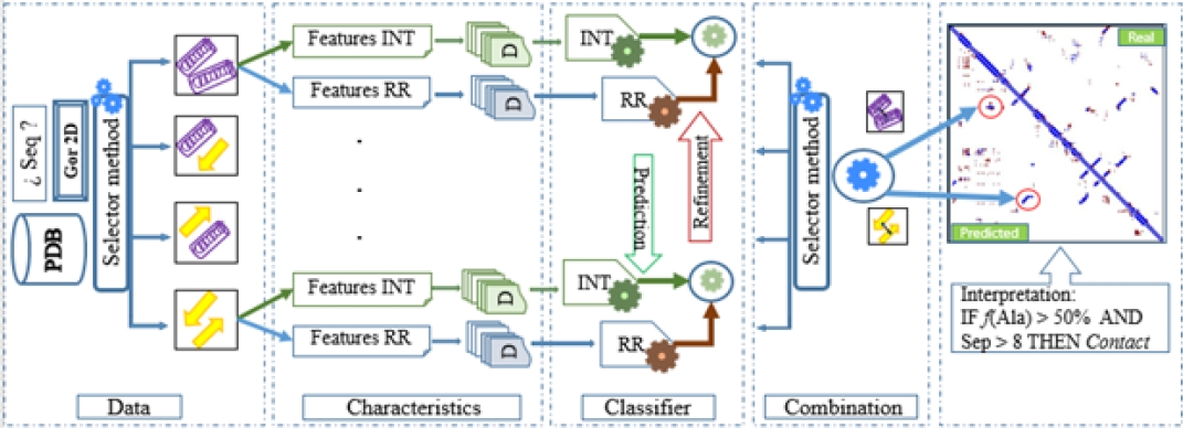
Fig. 1. Proposed predictor scheme. Where the rolls represent interactions between α-α structures, the yellow arrows represent β-β interactions
A construction strategy of multiple classifiers is constituted by four levels; which are, data, characteristics, classifiers, and the combination of results [26]. The method implemented in this article makes particular use of these levels to reach the final contact map. In the first level (data), it is common for contact prediction methods to use information from different sources such as multiple alignments [27], sequence profile [20].
For our modeling of the problem, a set of proteins with known secondary structure are extracted from the PDB (if not known the secondary structure can be calculated by a 2D predictor). Then, a selector process is applied to create disjoint datasets for each type of interaction between secondary structures (α-α, α/β, α+β, β-β, α-coil, coil-α, β-coil). This selector process ensures that the problem will be divided in sub-problems, then each multiple base classifier specializes in one sub-problem problem. In this way, it is possible to learn specific patterns for each type of interaction, which eventually results in specific rules to describe the folding which is novel for the prediction of contact maps.
At level two (characteristics), two different sets of descriptive features are used to create the training instances, (a) to describe the interactions between secondary structures and (b) to describe the inter-residual contacts that belong to such interactions.
Then with these instances the training sets are created (8 for interactions between secondary structures and 8 for inter-residual contacts). In addition, each training set for a specific multiple classifier pass through a sampling process explain in Fig. 2. This process ensures the diversity in the multiple classifier. Level three (classifiers), with the data sets previously created, each pair of multiple classifiers specialized in predicting and coding (or refining) of interaction are trained. he combined fashion to predict all referring to the interaction combines advantages of both structural and inter-residual steps such as the first is better detecting non-local interactions [15]. On the other hand, the second conveys strong information of the 3D model [12].
Finally, at level four (combination), there are different ways to combine the individual predictions of the base classifiers (in our case multiple classifiers). Where, in our proposal happen several operations, first, it is predicted if there is contact between secondary structures, this decision is taken by means majority vote of the multiple classifier dedicated to this task. Subsequently, the process of refinement occurs, where it is predicted that a pair of amino acids may be in contact within the interaction, also by means majority vote. Once interactions between secondary structures are predicted and refined, they are integrated into the final contact map, to do this we opted for a combination method [28], due to each pair of multiple classifiers dedicated to predict and refine the interactions know a part of the problem.
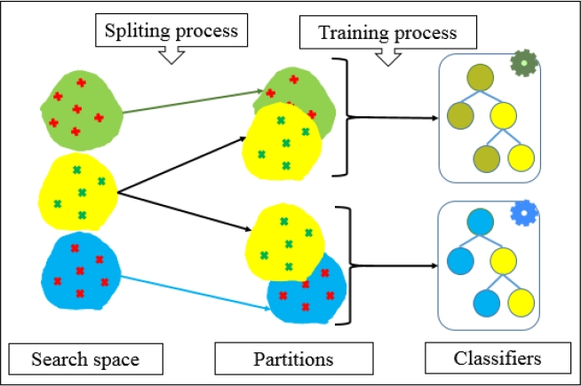
2.3 Training of a Base Multiple Classifier
Each of the multiple base classifiers employed in the proposal applies this training process, see Fig. 2. The intent of this process is; (1) to deal with one of the major challenges in the prediction problem of protein contact maps which is to solve the cost of predicting the positive class which is at least 1/60 with respect to negative class. And (2), guarantee the diversity of the base classifiers, which is a characteristic that must be met by all multiple classifiers.
To achieve these two objectives, a pre-processing of the total data set was applied, which was divided into negative and positive cases (non-contact and contact class respectively). Subsequently, the negative cases were divided into K partitions by means sampling with replacement, where K is the number of classifiers in the specialized multiple classifiers (K is set by the user), finally, the positive cases are replicated into each of these K partitions.
In the state-of-the-art of contact maps, some methods are trained in a balanced fashion with 50% positives and 50% negatives [29] or introducing a probability factor to reduce the training set [19], that looks for reducing the learning cycles. In our case, we don’t reduce any positive instance from the training set because they are considering as restrictions. Furthermore, with respect to the sampling with replacement which is a procedure considered a key strength of some of the best classifiers in nowadays [30], combined with the fashion way that we treated the positive cases contributes to our multiple classifiers to know different combinations of the search space always focusing on the positive cases.
2.4 Encoding Features for Secondary Structures Interactions
In the state-of-the-art, the prediction of interaction between secondary structures has been treated as a classification problem [13]. In this article, to model the interaction of two structures, we coding each secondary structure to simplified as a unique entity (or item, Helix, Sheet or Coil), to this way we can assign attributes such as physical and chemical properties.
Then we propose an encoding vector based on several sets of features to describe the context where the interaction takes place. Given a pair of secondary structures, the output of the multiple classifier used to predict their interaction is Contact or Non-Contact. The training vector used as input for the multiple classifier contains a total of 206 mixed features.
Where, the traits extracted from a structure are in total 34 and are described as follows; Hydrophobicity distribution two inputs (number of hydrophobic residues, non-hydrophobic), Polarity distribution four inputs (number of polar, non-polar, acid, basic residues), Charge distribution five inputs (number of atoms of hydrogen, nitrogen, oxygen, sulfur, carbon) Size distribution two inputs (number of big, small residues), Residues frequency 20 inputs (one for each amino acid), length of the secondary structure in residues (one input). A total of 204 features are computed to overall interaction (the two structures and their neighborhood, ±1 structures). Finally, we add two inputs more, one for the Separation between structures (number of intermediate structures) and other for the interaction Class (Contact or Non-Contact).
2.5 Encoding Features for Inter-Residuals Interactions
The contact between two residues (i and j) within the polypeptide sequence may be conditioned by various physical and chemical properties related to the context of the residues [31]. We use a features vector to encode these properties, where a total of 128 inputs are computed to analyze each pair of residues and their neighborhood (i±5 and j±5). These features are summarized in Table 1.
Table 1 Description of the attributes used in the residue-encoding vector. Each interaction between considered residues have a set of these attributes
| Features | Description | Type | Entries |
|---|---|---|---|
| For each residue (i, j) and its neighborhoods (window ±5 residues) | |||
| Hydrophobicity | (Hydrophobic, Hydrophilic). | Nominal | 1 |
| Polarity | (Polar, No-Polar, Acid-, Basic+). | Nominal | 1 |
| Organic compound | (Aromatic, Aliphatic, Unknown Organic compound). | Nominal | 1 |
| Subtotal of features for a window | 33 | ||
| Subtotal of features for the two windows | 66 | ||
| For the interaction between (i, j) with the opposite residue’s neighborhoods | |||
| Residue i to j-1…5 and j+1…..5 | H-H , NH-NH, ?-? | Nominal | 10 |
| Residue i to j-1…5 and j+1…..5 | P-P, A-A, B-B, NP-NP, ? -? | Nominal | 10 |
| Residue i to j-1…5 and j+1…..5 | Ar-Ar, Al-Al, UC-UC, ? -? | Nominal | 10 |
| Residue j to i-1…5 and i+1…..5 | H-H, H-NH, NH-NH. | Nominal | 10 |
| Residue j to i-1…5 and i+1…..5 | P-P, A-A, B-B, NP-NP, ? -? | Nominal | 10 |
| Residue j to i-1…5 and i+1…..5 | Ar-Ar, Al-Al, UC-UC, ? -? | Nominal | 10 |
| Subtotal of features for an interaction | 60 | ||
| Total features for the two target residues and their neighborhoods | 126 | ||
| Separation | Number of residues between the target residues | Numeric | 1 |
| Contact Class | Class (Contact o Non-Contact) | Nominal | 1 |
| Total of features | 128 | ||
Legend. Hydrophobic (H), Hydrophilic (NH), Polar (P), No-Polar (NP), Acid- (A), Basic+ (B), Aromatic (Ar), Aliphatic (Al), Unknown Organic compound (UC), Different type (?-?)
2.6 Decision Trees
In our model, we use decision trees to predict patterns of secondary structures interaction and inter-residual interactions within each multiple specialized classifier, specifically the C4.5 [32] (with C=0.25 and M=4) algorithm implemented in Weka [33]. Even we experimentally prove other tree-based method, but we select the aforementioned by it “simplicity” and also in some research is used to predict inter-residues contact [32]. Overall, this paradigm was selected firstly, require relatively little effort from users for data preparation, we do not need (mandatory) to worry about normalizing the data. They are not sensitive to outliers since the splitting happens based on the proportion of samples within the split ranges and not on absolute values. In addition, they can handle categorical and numeric attributes which is important, because we employed a mixed feature vector as input to the multiple classifiers [34].
On other hand, decision trees without proper pruning or limiting its growth, they tend to over-fit the training data, making them weak predictors. So this disadvantage is considered by some authors, an advantage, where an unstable tool, combined into an ensemble, they can create some of the best binary classifiers [35]. To conclude one of the most interesting characteristics that incite us to opt to use decision trees in our model was that, they could generate rules helping experts to formalize their knowledge, in our case these rules form part of an interpretation mechanism of the protein folding process.
2.7 Evaluation Measures
One of the challenges present in the prediction of contact maps of protein structures is the cost of predicting the positive class (contact) with respect to the negative class (non-contact), due to imbalance that is present between classes where is devote to find 1 contact of each 60 non-contacts [36]. For that reason, it is a demand to use metrics that give an unbiased idea of the performance of the methods with respect to the positive class. This implies that it is necessary to use measures that reflect the performance of the methods in that class, penalizing the negative class.
Measures such as Precision and Sensitivity (or Recall) are commonly used in this case. In addition, can be used F-measure (or Fm) [37] which establishes a balance between the precision and the sensitivity, providing a general idea of the prediction in function of the negative class. The Z-score is calculated by means the analysis of how well the predictions carried out by the predictive model are distributed [9], and it is a quality index of the of the predictions made by the proposed method based on precision Eq.1:
where X is a value of the set of prediction values, μ and σ are the mean and the standard deviation for the set of predictions.
2.8 Datasets
In the prediction problem of protein contact maps, the data sets are composed of proteins of known structure, downloaded from the PDB [38]. In addition, with the intention that the predictive model is trained with various data, the selected proteins have a similarity level of less than 30%. Our model was subjected to internal and external validation, for the internal validation of the model we created a set of proteins (IVS), which were divided into eight subgroups according to their SCOP classification (4) [39] and for the length of their sequence (4), see complementary materials.
For the external validation of the implemented method, firstly, a training set was created with 30% of each subgroup of IVS proteins, and as a test set we used the set of target proteins of CASP11, which can be downloaded from the official competition page1.
One of the challenges faced by the methods of contact maps prediction is the imbalance between classes. The Fig. 3 shows the imbalance index in the sets of proteins used in the experiment before being divided by sequence length.
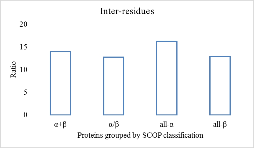
Fig. 3. shows the unbalance index (ratio), where the highest value is 15. As a reference, some studies show that this may be 60 (1/60 for contact / non-contact), [40]. One of the advantages of the proposed method is the natural ability to reduce the imbalance between inter-residues since the data used for training the classifiers employed to predict inter-residual interactions only use information from the structures that make contact, discarding all possible non-contact within structures that do not make contact.
3 Results and Discussion
3.1 Internal Validation
For the internal validation, the IVS data set and a cross-validation method (5x2) were used. In order to analyze the performance according to the domain application, the results are divided by SCOP classification of the proteins and by the length of the sequence. Table 2Table shows the average of the two executions for the metrics Precision, Sensitivity, and Fm.
Table 2 Experimental performance of the proposed algorithm predicting interactions between secondary structures in proteins with different sequence lengths
| Predictor Stages |
Ls < 100 | 100 ≤ Ls < 200 | 100 ≤ Ls < 200 | 300 ≤ Ls < 400 | Avg | |||||||||||||
|---|---|---|---|---|---|---|---|---|---|---|---|---|---|---|---|---|---|---|
| α+β | α/β | all-α | all-β | α+β | α/β | all-α | all-β | α+β | α/β | all-α | all-β | α+β | α/β | all-α | all-β | |||
| Secondary interactions | P | 0,73 | 0,90 | 0,69 | 0,65 | 0,76 | 0,77 | 0,73 | 0,70 | 0,74 | 0,74 | 0,77 | 0,77 | 0,74 | 0,72 | 0,80 | 0,71 | 0,75 |
| S | 0,74 | 0,89 | 0,68 | 0,66 | 0,78 | 0,80 | 0,75 | 0,72 | 0,77 | 0,77 | 0,79 | 0,80 | 0,78 | 0,75 | 0,83 | 0,74 | 0,77 | |
| Fm | 0,72 | 0,88 | 0,67 | 0,65 | 0,76 | 0,78 | 0,73 | 0,71 | 0,75 | 0,75 | 0,78 | 0,78 | 0,75 | 0,73 | 0,81 | 0,72 | 0,75 | |
| Inter-residues interactions | P | 0,41 | 0,49 | 0,15 | 0,51 | 0,49 | 0,52 | 0,23 | 0,43 | 0,43 | 0,42 | 0,4 | 0,55 | 0,42 | 0,4 | 0,46 | 0,45 | 0,42 |
| S | 0,31 | 0,32 | 0,21 | 0,32 | 0,34 | 0,37 | 0,34 | 0,31 | 0,35 | 0,34 | 0,35 | 0,38 | 0,29 | 0,29 | 0,36 | 0,28 | 0,32 | |
| Fm | 0,33 | 0,38 | 0,16 | 0,38 | 0,39 | 0,42 | 0,27 | 0,35 | 0,38 | 0,37 | 0,36 | 0,44 | 0,34 | 0,33 | 0,39 | 0,34 | 0,35 | |
Legend. The precision (P), Sensitivity (S) and Harmonic mean (Fm). Stratification of the sequence by length (Ls<100, 100≤Ls<200, 200≤Ls<300, 300≤Ls<400). Prediction of the secondary structure interaction, prediction of the inter-residues interactions
Table 2 shows the performance achieved by the method for the prediction of interactions between secondary structures and for the coding of residues that interact within these interactions. When analyzing the predictive capacity of interactions between secondary structures, the method achieves an average accuracy of 75%, with a maximum of 90% in α/β proteins. When we consider the SCOP classification of proteins, in general, our proposal performs better on α/β and all-α proteins, with a general average per group of 78% and 75%, respectively.
This suggests that the method is able to better interpret patterns of interaction between secondary structures in α-helix-dominated proteins. When we take into account the length of the sequence, the method reaches similar accuracy for all groups with an average of 76%. This is important since the method is not affected by increasing the sequence length, this due to the capacity to recognize local and non-local interactions.
When we analyze the Fm, we can verify the good performance of the method where the general average for this metric is 75%, which suggests the good balance between Precision and Sensitivity in terms of the prediction of interactions between secondary structures. Secondary structures interaction patterns differ with the topology of the protein [11], the performance of the implemented method shows that specializing can be a good way of dealing with this problem. Also, the unbiased prediction for local and non-local interactions can contribute to the prediction of long-range contacts.
The prediction of interactions between secondary structures is a crucial step for which our proposal obtains good results. The next step is to code such interactions by predicting inter-residual contacts. First, the general inter-residual prediction capacity (for the entire sequence) of the implemented method was analyzed. Where we take into account the SCOP classification, the best performance is reached in all-β proteins, with 49% accuracy (a state-of-art average standard [10]).
Several studies suggest that methods of predicting residues contact are able to learn better, patterns of inter-residual interaction from β-sheet structures [18], which is interesting for us since our method behaves similar to algorithms state-of-the-art (for this possibility), in addition, in these protein group our method reaches a maximum of 55% accuracy. Whereas, the worst performance in terms of precision for the prediction of inter-residual contacts is achieved in the set of all-α proteins, averaging 31%. Also, when the sequence length is taken into account, the performance achieved by the method is practically similar with an average of 43%, for the groups. Behavior that confirms that the sequence length does not affect the performance of the method.
As we can see, there is a difference between the contribution of the prediction at both the structural and inter-residual levels. Where at the inter-residual level it is difficult to the methods to understand that some parts of the context for some residues are feasibilities, for others are restrictions. Definitely, this drawback is better handled by the structural prediction level.
However, the method for all the inter residues contacts in the sequence performs practically similar for the entire domain of application.
3.1.1 Long-Range Contacts
Long-range contacts occur in a separation between residues of more than 24 residues in length. This type of contact is considered too complex to predict because inter-residual contacts decrease with increasing sequence separation, which implies a low number of patterns to recognize. To analyze the predictive capacity of the method implemented, we selected the results obtained in the internal validation for groups of proteins grouped by their SCOP classification and with a sequence length between 300 and 400 amino acids. Fig. 4 shows the precision results.
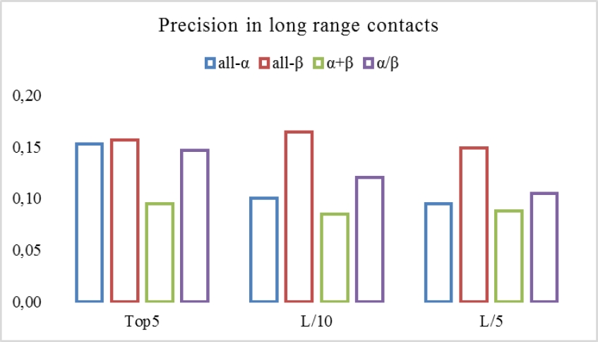
Fig. 4. Precision achieved by the method for long-range contacts (Top5, L/10, L/5, where L is the length of the sequence)
As Fig. 4 shows the method achieves a maximum precision value in 16% approximately. And we can note that best behaves is in Top5 long-range contacts. Even for Top5, the performance is similar for all-α and all-β protein groups. As we can observe in this figure, the precision values still low with respect to the precision values achieved for the all sequence contacts (Table 2), but the capacity of the method of having a similar behaves at least for all-α and all-β top5 contacts is a key-view of the generalization capability of our algorithm.
3.2 External Validation
In this analysis, we compare the long-range contact prediction capacity of our method with state-of-the-art well-ranked algorithms participating in the CASP11 competition. Taking into account the results presented by the official page competition, see complementary materials. Fig. 5 shows the precision and Z-score values for all the algorithms plus our method (SSIcm), in addition, with the intention to highlight the relation of both measures the results are sorted by the average of these metrics.
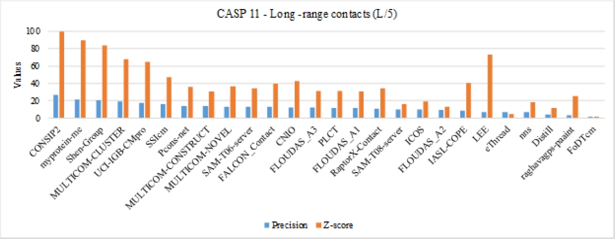
Fig. 5. Comparison of the proposed method with the CASP11 algorithms, the blue and orange bar are de precision and Z-score for the methods. The algorithm identification below in the y-axis is the ID related to the method’s name. Our method is labeled as SSIcm
As we can appreciate in Fig. 5, our method SSIcm does not achieve the best precision results, but even we note that our precision value is better than the values obtained by five well-known methods such as Distill (a method that consist in set of servers), eThread, nns, raghavagps-paaint or FoDTcm (which integrates a forest of decision trees). Whereas, in terms of Z-score our predictor have one of the highest results, overcome the majority of the methods. This means that our method can assign contacts with a high reliability. Taking into account the relation both metrics, we are ranked in the top-10, which suggests that the method can be competitive with some of the best methods of the state-of-the-art present in this competition.
3.3 Prediction Interpretation Mechanism
Understand the protein folding process is fundamental to Bioinformatics research field.
In this sense, our model can provide a set of rules (if-then-else) resulting from their prediction process. These rules describe the of proteins folding at different levels by means integrating the rules generated by both, the predictor of the secondary structure interaction and the inter-residual interaction, a small sample of these rules in shown in Fig. 6.

In the shown rules we can highlight characteristics of the interactions between secondary structures such as: the sub-sequence (SubSeq) existing between two secondary structures where elements such as the Small coils are important, as well as the separation between structures (Separation < 4).
Also, particularities of inter-residual interactions such as properties that the neighborhood of the target residues. In addition, threshold values for the residues belonging to the sub-sequence that is formed between i and j. At the end, these rules can be used in the developing drugs process as properties or requirements to be met [41], or as restrictions on the reconstruction of unknown or damaged proteins [42].
The mechanism employed to convert this set of rules in an interpretable expression is the same proposed in previous research [25]. Given the large volume of rules, it would be difficult to inspect them manually; therefore, it is possible to extract global statistics from the complete set of rules. In this sense, the rules were sorted by confidence level (top-down). Therefore, the most important rules must appear on the top. These rules became as easier and interpretable clues of the protein-folding process for the prediction of unknown structures.
4 Conclusions
After decades of intense research, the prediction of protein' contact maps still is a complicated problem which demands a deeper effort for researchers. In this article, we implement a novel model that employed decision trees and two steps (prediction and refining) of specialized context prediction to achieve the final contact map. In the first step intended to predict the secondary structure interaction, the method shows its suitability with an average precision of 75% and its capacity suitability for non-local interactions. Then in the second step, refining these interactions, the method was able to differentiate contact of non-contact with average 45% of precision for all the protein. Also, a comparison with algorithm participant in the CASP11 competition our method shows that is competitive with the state-of-the-art. An advantage of the model proposed is a mechanism to interpret the prediction which is useful to understand the protein folding process. In addition, the methods naturally reduce the imbalance between inter-residues classes.

