


Services on Demand
Journal
Article
 text in
  English (pdf)
 Article in xml format
 Article references
 Send this article by e-mail
Indicators
-
 Cited by SciELO
 -
 Access statistics
Related links
-
 Similars in
SciELO
Similars in
SciELO
Share

 Permalink
Agrociencia
On-line version ISSN 2521-9766Print version ISSN 1405-3195
Agrociencia vol.52 n.2 Texcoco Feb./Mar. 2018
Water-Soils-Climate
Fitting with L moments of the GVE, LOG and PAG distributions non-stationary in their location parameter, applied to extreme hydrological data
1Facultad de Ingeniería de la Universidad Autónoma de San Luis Potosí. Genaro Codina Núm 240. 78280 San Luis Potosí, San Luis Potosí. (campos_aranda@hotmail.com)
The analysis of frequencies of extreme hydrological data such as floods, droughts, winds and maximum daily precipitation, is based on accepting that the maximum annual data of the available sample are independent and come from a random process that is stationary. This means that their statistical properties do not vary with time. Due to changes in land use and impacts of global warming, the hydrological data series show trends, indicating that they are non-stationary. The objective of this study was to expose the generalization of the L moments method, to estimate the fit parameters of the probability distribution functions: General Extreme Values (GVE), Generalized Logistics (LOG) and Generalized Pareto (PAG) of non-stationary type, by varying with time (t) its location parameter (u) in a linear and quadratic way. The probabilistic models GVE1, LOG1 and PAG1 have four fitting parameters (δ1, δ2, a, k ), since u = δ1 + δ2·t and their scale (a) and form (k) parameters are constant. The models GVE2, LOG2 and PAG2 have five fitting parameters (δ1, δ2, δ3, a, k), due to the fact that u = δ1 + δ2·t + δ3·t2. In series with trend it is used as a covariate t in years, but indicators of regional or global climate variability can also be used, such as the southern oscillation index. By means of the four numerical applications that are described, the simplicity of the operating procedure was demonstrated and the utility of the use of non-stationary GVE, LOG and PAG models is highlighted through their predictions in series with trend, or using a climatic covariate.
Key words: L-moments; non-stationary probability distribution; linear regression; quadratic regression; standard error of fit; southern oscillation index
El análisis de frecuencias de datos hidrológicos extremos, como crecientes, sequías, vientos y precipitación máxima diaria, se basa en aceptar que los datos máximos anuales de la muestra disponible son independientes y provienen de un proceso aleatorio estacionario. Esto significa que sus propiedades estadísticas no varían en el tiempo. Debido a cambios en el uso del suelo e impactos del calentamiento global, las series de datos hidrológicos presentan tendencias, lo que indica que no son estacionarias. El objetivo de este estudio fue exponer la generalización del método de los momentos L, para estimar los parámetros de ajuste de las funciones de distribución de probabilidades: General de Valores Extremos (GVE), Logística Generalizada (LOG) y Pareto Generalizada (PAG) de tipo no estacionario, al variar con el tiempo (t) su parámetro de ubicación (u) de forma lineal y cuadrática. Los modelos probabilísticos GVE1, LOG1 y PAG1 tienen cuatro parámetros de ajuste (δ1, δ2, a, k), ya que u = δ1 + δ2·t y sus parámetros de escala (a) y forma (k) son constantes. Los modelos GVE2, LOG2 y PAG2 tienen cinco parámetros de ajuste (δ1, δ2, δ3, a, k), debido a que u = δ1 + δ2·t + δ3·t2. En series con tendencia se emplea como covariable t en años, pero también se pueden emplear indicadores de la variabilidad climática regional o global, como el índice de la oscilación del sur. Por medio de las cuatro aplicaciones numéricas que se describen, se demostró la sencillez del procedimiento operativo y la utilidad del uso de los modelos GVE, LOG y PAG no estacionarios se destacó a través de sus predicciones en series con tendencia, o usando una covariable climática.
Palabras clave: momentos L; distribuciones de probabilidad no estacionarias; regresión lineal; regresión cuadrática; error estándar de ajuste; índice de la oscilación del sur
Introduction
All the hydraulic works of use or control, such as reservoirs, protection dams, canalizations and rectifications, bridges and urban pluvial drainage, require in the stages of planning, design and operation of the estimate, as accurate as possible, of the design floods. Based on these hydrological estimates, hydraulic works are sized and an attempt is made to guarantee their safety; therefore, the design floods are predictions associated with low probabilities of exceedance, which are obtained through the Flood Frequency Analysis (AFC). There is another stage in which it is necessary to review the hydrological safety of hydraulic works, when one of the following two eventualities occurs: 1) it reached the end of its useful life and therefore there is more information to carry out the AFC; or, 2) changes have occurred in its basin, be these land use, construction of other hydraulic works or those caused by climate change (Jakob, 2013).
The AFC is a statistical technique of inference, which uses a probabilistic model or distribution function of probabilities (FDP), to represent the available sample of instantaneous annual maximum flows. This procedure encompasses the following five stages (Rao and Hamed, 2000; Meylan et al., 2012): 1) data collection and verification of their statistical quality, 2) selection of a FDP; 3) choice of a method for estimating its fit parameters, 4) objective quantification of the fit achieved with each FDP and estimation technique, and 5) selection of results.
The AFC is based on the assumption of stationarity, that is, of a climate that does not change with time in the statistical sense and for that reason, it is accepted that the available records of annual maximum flow are independent and are identically distributed, condition designated " iid." However, in recent years the global climate change caused by the increase in the effect of greenhouse gases has been accepted. These two physical considerations have generated an intensification of the hydrological cycle, with increases in frequency and intensity of extreme precipitation events and consequently, in the possibility of more severe floods (Katz, 2013; Kim et al., 2015; Álvarez-Olguín y Escalante-Sandoval, 2016).
The extension of the statistical theory of extreme values to the case of non-stationary hydrological records has followed approaches described by Khaliq et al. (2006). One of these approaches, perhaps the simplest one, applies the classical FDP of this theory, the General Distribution of Extreme Values (GVE) with three parameters (u, a, k), allowing a translate or fit gradual when introducing the time t as a covariate in its location parameter u, keeping constant that of the scale a and that of the form k (Park et al., 2011; Katz, 2013).
A nomenclature for these non-stationary FDPs has been established. El Adlouni et al. (2007) and Aissaoui-Fqayeh et al. (2011) defined the stationary GVE function as GVE0, which has its location parameter linearly variable with time (u = δ1 + δ2·t) as GVE1 and when the variation is quadratic (u = δ1 + δ2· t + δ3 · t2) is the GVE2. In the GVE11 model, the location and scale parameters vary linearly with time. In the models cited, another covariate that has been used is some indicator of global or regional climatic variability (López de la Cruz y Francés, 2014; Franks et al., 2015; Álvarez-Olguín y Escalante-Sandoval, 2016), as the Southern Oscillation Index (SOI). SOI is quantified as the difference in surface air pressure between Darwin, Australia and Tahiti in French Polynesia (Teegavarapu, 2012).
The objective of this study was to present in detail the generalization of the L-moments method to estimate the fitting parameters of the FDPs non-stationary GVE1 and GVE2, which was proposed, applied and contrasted by El Adlouni and Ouarda (2008b), using as covariables, time t and SOI. This procedure was extended to the FDPs Generalized Logistics (LOG) and Generalized Pareto (PAG), which are models used in the analysis of frequencies of extreme hydrological data (Kim et al., 2015) Four numerical applications are described with data from the specialized literature and the simplicity and usefulness of the L-moments method for the fit of the six non-stationary FDPs exposed is highlighted.
Materials and Methods
Populations and sample L-moments
The L-moments are an alternative system to describe the forms of the FDP. Historically they appear as modifications of the weighted probability moments (MPP) developed by Greenwood et al. (1979). The MPPs of a random variable x with accumulated FDP F(x) were defined by the following quantities:
Of particular interest is the following special case: βr = M1,r,0. For a distribution with function of quantiles x(F), equation 1 leads to:
This equation can be contrasted with the ordinary definition of the moments, that is:
The conventional definition of moments involves successive powers of the quantile function x(F), while the MPPs involve successive powers of F and therefore can be considered as integrals of x(F) weighted by polynomials Fr ; hence its name. MPPs substantially improve the properties of sampling, as they are not influenced by scattered values (Asquith, 2011). The L-moments are linear combinations of the MPPs, as follows (Hosking and Wallis, 1997):
In addition, the quotients (τ) of L-moments are defined, starting with L -Cv which is analogous to this coefficient and then those of similarity with the coefficients of asymmetry and kurtosis, these are:
In a sample of size n, with its elements in ascending order (x1 ≤ x2 ≤… xn) the unbiased estimators of βr are (Stedinger et al., 1993; Hosking and Wallis, 1997) are:
with the following general expression:
The sampling estimators of λr will be lr being defined by equations 4 a 7 and those of the ratios of L-moments will be t, t3 and t4, according to equations 8 to 10.
Fitting with L-moments of the distributions GVE, LOG, and PAG
Hosking and Wallis (1997) highlighted in their “Table 5.1”, that these three FDPs, when their shape parameter is negative (k < 0), have their right tails thicker or denser than all other FDPs commonly used in the AFC; due to this they have gained acceptance in the analysis of frequencies of extreme hydrological data (El Adlouni et al., 2008a). These three PDFs also coincide in having an upper limit when k > 0 and defining functions of two fit parameters known as Gumbel, Logistics and Exponential, when k = 0.
Next, the inverse solution x(F) for the GVE, LOG and PAG distributions is cited, with which the predictions associated with a certain probability of non-exceedance (F) are estimated and the equations that allow us to estimate their three fit parameters (u, a, k) corresponding to the location, scale and form, with the method of L-moments.
Distribution GVE (Hosking and Wallis, 1997): interval of x: u + a/k ≤ x < ∞ si k < 0; - ∞< x < ∞ si k = 0; - ∞ < x ≤ u + a/k si k > 0.
being:
For the evaluation of the Gamma function the Stirling formula (Davis, 1972) was used:
Distribution LOG (Hosking and Wallis, 1997): interval of x, identical to that of the GVE.
For distribution PAG (Hosking and Wallis, 1997) the interval of x is u ≤ x < ∞ if k ≤ 0; u ≤ x ≤ u + a/k if K > 0.
Fitting with L-moments of the distribution GVE1 and GVE2
The generalization of the L-moments method proposed by El Adlouni and Ouarda (2008b) for the fitting of the non-stationary FPD type GVE1 begins by analyzing the expected value according to the expression:
From this equation it is deduced that an estimator
It is deduced from equation 29, that the new variable is distributed according to a FDP type GVE0 with parameters δ1, a and k that are estimated with equations 16 to 19 of the L-moments method, highlighting that u (equation 19) is equal to δ1, with which the four fitting parameters of the GVE1 model are estimated. Equation 30 corresponds to one of the first simple approaches suggested to process hydrological records with tendency, consisting in removing first such a deterministic component (McCuen and Thomas, 1990, Campos-Aranda, 2012). As Mudersbach and Jensen (2010) have indicated, such an approach is practical but the results of its AFC are valid only in the present and hydraulic works must be safe at the end of their useful life, requiring that the flood of design be estimated in a predetermined future date.
The same approach is used to introduce a quadratic dependence on the location parameter
u, therefore, the estimates
With the equations 16 to 19 applied to the corrected data sample S2, the remaining parameters k, a and δ1 of the GVE2 model are defined. El Adlouni and Ouarda (2008b) compared by numerical simulation three procedures for obtaining the four and five fitting parameters of the GVE1 and GVE2 models: the maximum likelihood method (Coles, 2001, Nadarajah, 2005, Katz, 2013), generalized maximum likelihood (Martins and Stedinger, 2000; El Adlouni et al., 2007) and their generalization of the L-moments; they conclude that the latter is better than the first, because it has lower bias and mean square error, but it does not exceed the second, especially in records with important asymmetry.
Equations of linear regression
It is considered that the dependent variable (y) are the annual hydrological data Xi and the times or years ti are the abscissas (x), in this case equal to the i-th value i. To test if the slope (δ2) of the regression line fitted by least squares of the residuals, is statistically different from zero, a test based on the Student's distribution (DS) defined by the following equations was used (Ostle and Mensing, 1975):
where:
G1 = (Z3 + Z)/4
G2 = (5Z5 +16Z3 + 3Z)/96
G3 = (3Z7 + 19Z5 + 17Z3 - 15Z)/384
G4 = (79Z9 + 776Z7 + 1482Z5 - 1920Z3 - 945Z)/92160
Slope δ2 according to the Pranab Kumar Sen criterion
To verify numerically the value obtained from δ2 with equation 34, the Sen criterion (1968) was used, which utilizes the formula of the trend established in the Kendall test, to estimate its slope, defining it as the median value (MED) of the partial slopes, that is:
Xj and Xi are the data in the j and i times, which represent years: being n the number of data, then we have n(n - 1)/2 partial slopes. δ2 has units of X/year and its positive sign defines ascending tendencies and negative descending ones. Machiwal and Jha (2012) indicate that this criterion is resistant or robust to the presence of scattered values (outliers).
Equations of the quadratic regression
The quadratic or parabolic polynomial for the nonlinear trend between the Xi data and the years of the ti record is (Campos-Aranda, 2003):
whose matrix arrangement of its normal equations is:
with solution:
being, T a square matrix with inverse T-1, δ a vector column of unknowns and X another vector column of independent terms. The coefficient of determination R2 quantifies the degree of correlation of the polynomial fitting, its numerator measures the improvement or reduction of the error due to the regression and its denominator is the dispersion of the dependent variable, that is:
Being:
Since Se2 is always smaller than Sx2, then R2 varies from zero to unity (when Se2 = 0) and its square root corresponds to the coefficient of polynomial correlation (Campos-Aranda, 2003).
Fitting with L-moments of the distributions LOG1, LOG2, PAG1, and PAG2
In Rao and Hamed (2000) the equations of the expected value of the Generalized Logistics (LOG) and Generalized Pareto (PAG) distributions can be found, similar to the expression 29 of the GVE function. This implies that the generalization of El Adlouni and Ouarda (2008b) of the L-moments method to fit non-stationary FDP with variable location parameter in time is also applicable in the LOG and PAG models.
Standard error of fit
In the mid-1970s the standard error of fit (EEA) was established as a quantitative statistical indicator, since it evaluates the standard deviation of the differences between the observed values and those estimated with the FDP that is tested; in this study the models: GVE1, GVE2, LOG1, LOG2, PAG1 and PAG2. Their expression is as follows (Kite, 1977, Pandey and Nguyen, 1999):
in which, n and np are the number of the sample data and of fitting parameters, in this case four and five; Xi are the ordered data from least to greatest and are estimated values with the inverse solution x(F) or quantile function that uses the variable location parameter, for a probability of non-exceedance estimated with the Weibull formula (Benson, 1962):
where, m is the data order number, with 1 for the smallest and n for the largest one.
Records of annual maximum values to be processed
Four records of the specialized literature were selected to illustrate the application of the non-stationary FDPs GVE, LOG and PAG with the generalization method of the L-moments (El Adlouni and Ouarda, 2008b); their values are shown in Table 1. These records have approximate data read in the graphs where they were exposed. The first record was shown by Leclerc and Ouarda (2007) as an example of a series of flows (m3·s-1) with a downward trend in a hydrometric station of the Dartmouth River in Canada, with 630 km2 of basin area. The second record is the annual daily maximum precipitation (PMD) in millimeters corresponding to the Andong rainfall station in South Korea (Park et al., 2011) and was selected for its strong upward trend.
Table 1 Maximum annual data to be processed of flow (Q), maximum daily precipitation (PMD) and southern oscillation index (SOI) in the indicated stations.
| No. | Dartmouth | Andong | Ficticia | Tehachapi | |||||
| Año | Q | Año | PMD | Año | PMD | Año | PMD | SOI | |
| 1 | 1974 | 154 | 1973 | 60 | 1961 | 16.0 | 1952 | 15 | -0.2 |
| 2 | 1975 | 227 | 1974 | 67 | 1962 | 18.6 | 1953 | 17 | 0.8 |
| 3 | 1976 | 217 | 1975 | 120 | 1963 | 10.0 | 1954 | 13 | 0.9 |
| 4 | 1977 | 398 | 1976 | 76 | 1964 | 10.4 | 1955 | 38 | -0.7 |
| 5 | 1978 | 238 | 1977 | 87 | 1965 | 10.5 | 1956 | 29 | -0.6 |
| 6 | 1979 | 244 | 1978 | 27 | 1966 | 8.3 | 1957 | 45 | -0.3 |
| 7 | 1980 | 150 | 1979 | - | 1967 | 8.1 | 1958 | 21 | 0.5 |
| 8 | 1981 | 346 | 1980 | - | 1968 | 10.5 | 1959 | 37 | 1.2 |
| 9 | 1982 | 223 | 1981 | - | 1969 | 13.3 | 1960 | 24 | 0.2 |
| 10 | 1983 | 180 | 1982 | - | 1970 | 10.2 | 1961 | 36 | -0.9 |
| 11 | 1984 | 145 | 1983 | 129 | 1971 | 9.6 | 1962 | 16 | -0.6 |
| 12 | 1985 | 122 | 1984 | 121 | 1972 | 9.2 | 1963 | 25 | 0.4 |
| 13 | 1986 | 99 | 1985 | 88 | 1973 | 15.5 | 1964 | 12 | -0.3 |
| 14 | 1987 | 198 | 1986 | 82 | 1974 | 12.5 | 1965 | 36 | 0.7 |
| 15 | 1988 | 191 | 1987 | 87 | 1975 | 9.2 | 1966 | 17 | 0.4 |
| 16 | 1989 | 129 | 1988 | 78 | 1976 | 22.3 | 1967 | 16 | -0.5 |
| 17 | 1990 | 214 | 1989 | 62 | 1977 | 13.4 | 1968 | 56 | -0.2 |
| 18 | 1991 | 195 | 1990 | 69 | 1978 | 9.5 | 1969 | 35 | -1.1 |
| 19 | 1992 | 173 | 1991 | 100 | 1979 | 13.2 | 1970 | 36 | 0.6 |
| 20 | 1993 | 101 | 1992 | 75 | 1980 | 13.0 | 1971 | 13 | -0.2 |
| 21 | 1994 | 159 | 1993 | 114 | 1981 | 8.6 | 1972 | 34 | -0.5 |
| 22 | 1995 | 148 | 1994 | 69 | 1982 | 7.8 | 1973 | 42 | -0.4 |
| 23 | 1996 | 158 | 1995 | 109 | 1983 | 10.3 | 1974 | 17 | 1.5 |
| 24 | 1997 | 225 | 1996 | 90 | 1984 | 9.0 | 1975 | 18 | 1.4 |
| 25 | 1998 | 175 | 1997 | 119 | 1985 | 8.6 | 1976 | 31 | -0.8 |
| 26 | 1999 | 275 | 1998 | 114 | 1986 | 16.1 | 1977 | 21 | 2.1 |
| 27 | 2000 | 144 | 1999 | 97 | 1987 | 10.1 | 1978 | 17 | 0.1 |
| 28 | 2001 | 192 | 2000 | 170 | 1988 | 9.2 | 1979 | 19 | 1.4 |
| 29 | 2002 | 65 | 2001 | 94 | 1989 | 15.3 | 1980 | 41 | -0.1 |
| 30 | 2003 | 142 | 2002 | 115 | 1990 | 13.5 | 1981 | 82 | -1.4 |
| 31 | - | - | 2003 | 103 | 1991 | 12.2 | 1982 | 18 | -0.2 |
| 32 | - | - | 2004 | 129 | 1992 | 12.7 | 1983 | 45 | -0.5 |
| 33 | - | - | 2005 | 77 | 1993 | 10.3 | 1984 | 35 | -0.6 |
| 34 | - | - | 2006 | 102 | 1994 | 19.9 | 1985 | 19 | 0.3 |
| 35 | - | - | 2007 | 89 | 1995 | 19.6 | 1986 | 87 | -3.2 |
| 36 | - | - | - | - | 1996 | 13.9 | 1987 | 29 | -0.2 |
| 37 | - | - | - | - | 1997 | 15.8 | 1988 | 28 | 0.1 |
| 38 | - | - | - | - | 1998 | 13.7 | 1989 | 29 | -0.2 |
| 39 | - | - | - | - | 1999 | 16.7 | 1990 | 19 | -1.5 |
| 40 | - | - | - | - | 2000 | 15.7 | 1991 | 22 | -0.4 |
| 41 | - | - | - | - | 2001 | 18.7 | 1992 | 16 | 1.2 |
| 42 | - | - | - | - | 2002 | 21.9 | 1993 | 17 | -0.8 |
| 43 | - | - | - | - | 2003 | 18.8 | 1994 | 41 | -0.4 |
| 44 | - | - | - | - | 2004 | 30.0 | 1995 | 48 | -1.9 |
| 45 | - | - | - | - | 2005 | 22.1 | 1996 | 49 | -0.9 |
| 46 | - | - | - | - | 2006 | 17.2 | 1997 | 26 | -0.3 |
| 47 | - | - | - | - | 2007 | 22.6 | 1998 | 71 | -0.6 |
| 48 | - | - | - | - | 2008 | 18.7 | 1999 | 33 | 0.2 |
| 49 | - | - | - | - | 2009 | 22.2 | 2000 | 27 | 0.3 |
| 50 | - | - | - | - | 2010 | 22.6 | - | - | - |
The third record comes from El Adlouni and Ouarda (2008b) and they are randomly generated data with a GVE2 distribution whose values in their fitting parameters were: δ1 = 10, δ2 = -0.10, δ3 = 0.005, a = 1.0 and k = -0.10; corresponds to a PMD series with nonlinear trend. The fourth record also comes from the previous reference and has been used by El Adlouni et al. (2007), Aissaoui-Fqayeh et al. (2009) and Ouarda and El Adlouni (2011), corresponds to the PMD recorded in the period from 1952 to 2000 at the Tehachapi rainfall station in Southern California, U.S.A. These values are related to the SOI (Southern Oscillation Index) and, therefore, they will be used as a covariate.
General layout for probabilistic analysis
The graph of data values (Xi ) versus time (ti ) allows defining if there is a linear or quadratic trend. When the trend is linear, the fitting parameters (δ2, δ1, a, k) of the non-stationary FDPs GVE1, LOG1 and PAG1 are estimated, their EEA is quantified with equation 48, to select the FPD that leads to the lowest value of such indicator. When the trend is curved, the non-stationary PDFs the GVE2, LOG2 and PAG2 are tested; for this, their fitting parameters are estimated (δ2, δ3, δ1, a, k), their EEA is quantified, adopting the one that contributed the lowest value. In this process, a non-stationary FDP can be adopted, based on judgments of convenience, for example, the most unfavorable or critical predictions. The above is illustrated in the first numerical application.
In the analyses that use time (t) as a covariate, based on the inverse solutions (equations 15, 21 and 25) of the GVE, LOG and PAG distributions, predictions with return periods (Tr) of 2, 25, 50 and 100 years were calculated, through the registration period, the location parameter variable u was applied. The first prediction corresponds to the median, since its probability of non-exceedance (F) is 50 % and the following three are calculated for complementary probabilities, to define its superior and inferior value (Park et al., 2011), that is, for the following values: F = 0.96 and F = 0.04 for the Tr of 25 years; F = 0.98 and F = 0.02 for the Tr of 50 years and F = 0.99 and F = 0.01 for the Tr of 100 years. Furthermore, in these analyses, predictions were made for the future, in the years 2020, 2050 and 2100. When the covariate is the SOI, the predictions corresponding to the Tr of 2, 25, 50 and 100 years, fluctuate according to the magnitude of the SOI and then its maximum values are indicated in the extreme magnitude of the SOI. In this case, future predictions are possible using prognostic SOI values.
Results and Discussion
Predictions at a Dartmouth River gauging station
These data show a linear descent and significant trend, since DS= -2.2931 and DSc = 2.0484 (Figure 1). In this record, the EEAs of the non-stationary FDPs GVE1, LOG1 and PAG1 are 42.0, 43.1 and 41.6 m3·s-1. Due to the numerical similarity that the EEA have, the results of the function LOG1 are adopted because they lead to the largest or most critical predictions. Their fitting parameters are δ2 = -3.125, δ1 = 227.919, a = 33.318 and k = -0.144; with a linear correlation coefficient of -0.3976 and a slope of -2.8182 as Sen criterion. Table 2 shows some of the predictions within the record and in the future on three pre-fixed dates. This record of 30 data ends in 2003, therefore, the value of time t in 2020 is 47, in 2050 it is 77 and in 2100 it was 127.
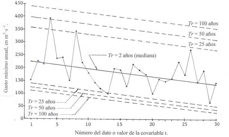
Figure 1 Diagram of data and rights of predictions estimated with the LOG1 distribution in a hydrometric station of the Dartmouth River, Canada.
Table 2 Predictions (m3·s-1) in the historical period and in the future in a hydrometric station of the Dartmouth River, based on the non-stationary FDP LOG1.
| No. (t) | Año | Gasto (Q) | Tr†= 2 años | Tr = 25 años | Tr = 50 años | Tr = 100 años | |||
| (Mediana) | VS¶ | VI§ | VS | VI | VS | VI | |||
| 1 | 1974 | 154 | 224.8 | 359.1 | 139.8 | 398.7 | 125.5 | 441.8 | 112.8 |
| 10 | 1983 | 180 | 196.7 | 330.9 | 111.7 | 370.5 | 97.4 | 413.7 | 84.7 |
| 20 | 1993 | 101 | 165.4 | 229.7 | 80.5 | 339.3 | 66.2 | 382.5 | 53.4 |
| 30 | 2003 | 142 | 134.2 | 268.4 | 49.2 | 308.0 | 34.9 | 351.2 | 22.2 |
| No. (t) | Año | uÞ | Tr = 2 años | Tr = 25 años | Tr = 50 años | Tr = 100 años | |||
| (Mediana) | VS | VI | VS | VI | VS | VI | |||
| 47 | 2020 | 81.0 | 81.0 | 215.3 | 0.0 | 254.9 | 0.0 | 298.1 | 0.0 |
| 77 | 2050 | -12.7 | -12.7 | 121.6 | 0.0 | 161.2 | 0.0 | 204.3 | 0.0 |
| 127 | 2100 | -169.0 | -169.0 | 0.0 | 0.0 | 4.9 | 0.0 | 48.1 | 0.0 |
†Return period. ¶Higher value. §Lower value. Þlocation parameter.
Predictions at the Andong pluviometric station
This PMD record has a linear upward and significant trend, because DS = 2.1568 and DSc = 2.0452 (Figure 2). The fitting of the non-stationary PDFs GVE1, LOG1 and PAG1 led to the following EEAs in millimeters: 9.8, 8.8 and 11.9. For this record the LOG1 function is adopted, for achieving the lowest EEA, its fitting parameters were: δ2 = 1.1101, δ1 = 73.805, a = 13.740 and k = -0.113; with a linear correlation coefficient of 0.3718 and a slope of 1.100 according to the Sen criterion. Table 3, lists a part of the predictions within the record and in the future on three pre-fixed dates. As this record covers 31 data and concludes in 2007, the magnitude of time t in 2020 is 44, in 2050 it is 74 and in 2100 it was 124.
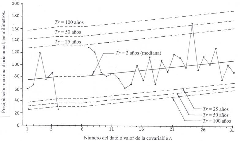
Figure 2 Diagram of data and predictions estimated with the distribution LOG1 in the pluviometric station Andong, South Korea.
Table 3 Predictions (mm) in the historical period and in the future in the Andong pluviometric station, based on the non-stationary FDP LOG1
| No. (t) | Año | PMD | Tr†= 2 años | Tr = 25 años | Tr = 50 años | Tr = 100 años | |||
| (Mediana) | VS¶ | VI§ | VS | VI | VS | VI | |||
| 1 | 1973 | 60 | 74.9 | 127.5 | 38.2 | 142.1 | 31.7 | 157.7 | 25.7 |
| 10 | 1986 | 82 | 84.9 | 137.5 | 48.2 | 152.1 | 41.7 | 167.7 | 35.7 |
| 20 | 1996 | 90 | 96.0 | 148.6 | 59.3 | 163.2 | 52.8 | 178.8 | 46.8 |
| 31 | 2007 | 89 | 108.2 | 160.8 | 71.5 | 175.4 | 65.0 | 191.0 | 59.0 |
| No. (t) | Año | uÞ | Tr = 2 años | Tr = 25 años | Tr = 50 años | Tr = 100 años | |||
| (Mediana) | VS | VI | VS | VI | VS | VI | |||
| 44 | 2020 | 122.6 | 122.6 | 175.2 | 86.0 | 189.8 | 79.4 | 205.4 | 73.4 |
| 74 | 2050 | 156.0 | 156.0 | 208.5 | 119.3 | 223.1 | 112.7 | 238.8 | 106.7 |
| 124 | 2100 | 211.5 | 211.5 | 264.0 | 174.8 | 278.6 | 168.2 | 294.3 | 162.2 |
†Return period. ¶Higher value. §Lower value. ÞLocation parameter.
Predictions in a pluviometric fictitious station
This PMD record has an upward curve trend (Figure 3). The fitting of the non-stationary PDFs GVE2, LOG2 and PAG2 led these values of the EEA in millimeters: 2.4, 2.3 and 2.5. The LOG2 function is adopted to achieve the lowest EEA; its fitting parameters were: δ2 = -0.3367, δ3 = 0.0109, δ 1 = 12.828, a = 1.618 and k = -0.264, with a polynomial correlation coefficient of 0.715. Table 4 shows a part of the predictions within the record and in future in three pre-fixed dates. This record of 50 data ends in the year 2010, then the magnitude of time t in 2020 is 60, in 2050 it is 90 and in 2010 it was 140.
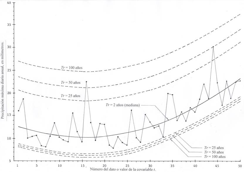
Figure 3 Diagram of data and curves of prediction estimated with the distribution LOG2, in a fictitious pluviometric station.
Table 4 Predictions (mm) in the historic period and in future in the fictitious pluviometric station, based on the non-stationary FDP LOG2.
| No. (t) | Año | PMD | Tr†= 2 años | Tr = 25 años | Tr = 50 años | Tr = 100 años | |||
| (Mediana) | VS¶ | VI§ | VS | VI | VS | VI | |||
| 1 | 1961 | 16.0 | 12.5 | 20.6 | 9.0 | 23.5 | 8..6 | 27.0 | 8.2 |
| 10 | 1970 | 10.2 | 10.5 | 18.6 | 7.1 | 21.6 | 6.6 | 25.1 | 6.2 |
| 20 | 1980 | 13.0 | 10.4 | 18.5 | 7.0 | 21.4 | 6.5 | 24.9 | 6.1 |
| 30 | 1990 | 13.5 | 12.5 | 20.6 | 9.0 | 23.5 | 8.6 | 27.0 | 8.2 |
| 40 | 2000 | 15.7 | 16.8 | 24.8 | 13.3 | 27.8 | 12.8 | 31.3 | 12.5 |
| 50 | 2010 | 22.6 | 23.2 | 31.2 | 19.7 | 34.2 | 19.2 | 37.7 | 18.9 |
| No. (t) | Año | uÞ | Tr = 2 años | Tr = 25 años | Tr = 50 años | Tr = 100 años | |||
| (Mediana) | VS | VI | VS | VI | VS | VI | |||
| 60 | 2020 | 31.8 | 31.8 | 39.8 | 28.3 | 42.8 | 27.8 | 46.3 | 27.5 |
| 90 | 2050 | 70.6 | 70.6 | 78.7 | 67.1 | 81.6 | 66.7 | 85.1 | 66.3 |
| 140 | 2100 | 178.8 | 178.8 | 186.9 | 175.3 | 189.8 | 174.9 | 193.3 | 174.5 |
†Return period. ¶Higher value. §Lower Value. ÞLocation parameter.
Predictions in the pluviometric station Tehachapi
Figure 4 shows the annual PMD record is shown in the ordinates against their corresponding values of the SOI on the abscissa, since it is not possible to select between a linear descending trend or a curve, the two fits will be applied. The non-stationary PDFs GVE1, LOG1 and PAG1 lead to the following values of the EEA in millimeters: 11.6, 11.4 and 12.2. For this linear fitting, the LOG1 function is adopted for achieving the lowest EEA; its fitting parameters were: δ2 = -10.2657, δ1 = 28.376, a = 7.570 and k = -0.104, with a linear correlation coefficient of -0.5680. Table 5 shows a part of the prediction within the record.
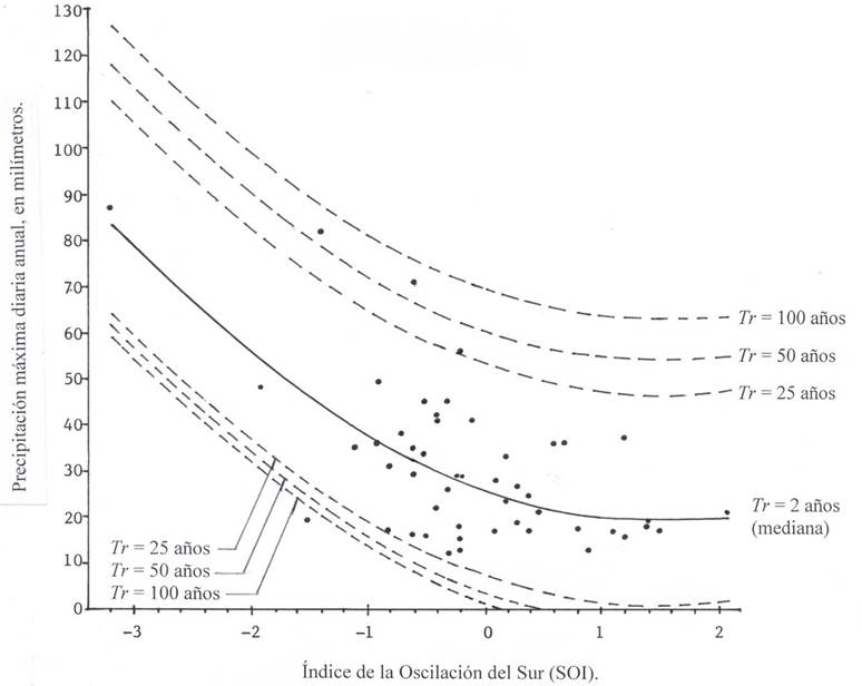
Figure 4 Estimated prediction curves with the LOG2 distribution in the Tehachapi pluviometric station in Southern California, U.S.A.
Table 5 Predictions (mm) in the historic period in the pluviometric station Tehachapi, based on the non-stationary FDP LOG1.
| Datos | Tr†= 2 años | Tr = 25 años | Tr = 50 años | Tr = 100 años | |||||
| No. | SOI | PMD | (Mediana) | VS¶ | VI§ | VS | VI | VS | VI |
| 26 | 2.1 | 21 | 6.8 | 35.3 | 0.0 | 43.1 | 0.0 | 51.4 | 0.0 |
| 23 | 1.5 | 17 | 13.0 | 41.5 | 0.0 | 49.3 | 0.0 | 57.5 | 0.0 |
| 3 | 0.9 | 13 | 19.1 | 47.6 | 0.0 | 55.4 | 0.0 | 63.7 | 0.0 |
| 7 | 0.5 | 21 | 23.2 | 51.7 | 2.7 | 59.5 | 0.0 | 67.8 | 0.0 |
| 29 | -0.1 | 41 | 29.4 | 57.9 | 8.9 | 65.7 | 5.2 | 73.9 | 1.7 |
| 30 | -1.4 | 82 | 42.7 | 71.2 | 22.2 | 79.0 | 18.5 | 87.3 | 15.1 |
| 44 | -1.9 | 48 | 47.9 | 76.4 | 27.4 | 84.2 | 23.6 | 92.4 | 20.2 |
| 35 | -3.2 | 87 | 61.2 | 89.7 | 40.7 | 97.5 | 37.0 | 105.8 | 33.5 |
†Return period ¶Higher value. §Lower value.
The non-stationary FDPs GVE2, LOG2 and PAG2 lead to the following values of the EEA in millimeters: 12.8, 12.7 and 13.3. For this non-linear fitting, the LOG2 function is adopted, to achieve the lowest EEA value; its fitting parameters were: δ2 = -8.7385, δ3 = 2.8432, δ1 = 25.936, a = 6.942 and k = -0.127, with a polynomial correlation coefficient of 0.6279. Table 6 shows a part of the predictions within the record.
Table 6 Predictions (mm) in the historic period in the pluviometric station Tehachapi, based on the non-stationary FDP LOG2.
| Datos | Tr†= 2 años | Tr = 25 años | Tr = 50 años | Tr = 100 años | |||||
| No. | SOI | PMD | (Mediana) | VS¶ | VI§ | VS | VI | VS | VI |
| 26 | 2.1 | 21 | 20.1 | 47.3 | 2.0 | 55.0 | 0.0 | 63.4 | 0.0 |
| 23 | 1.5 | 17 | 19.2 | 46.4 | 1.1 | 54.1 | 0.0 | 62.5 | 0.0 |
| 3 | 0.9 | 13 | 20.4 | 47.5 | 2.2 | 55.3 | 0.0 | 63.7 | 0.0 |
| 7 | 0.5 | 21 | 22.3 | 49.4 | 4.1 | 57.2 | 1.0 | 65.6 | 0.0 |
| 29 | -0.1 | 41 | 26.8 | 54.0 | 8.7 | 61.8 | 5.5 | 70.1 | 2.7 |
| 30 | -1.4 | 82 | 43.7 | 70.9 | 25.6 | 78.7 | 22.4 | 87.0 | 19.6 |
| 44 | -1.9 | 48 | 52.8 | 80.0 | 34.6 | 87.7 | 31.5 | 96.1 | 28.6 |
| 35 | -3.2 | 87 | 83.0 | 110.2 | 64.9 | 117.9 | 61.7 | 126.3 | 58.8 |
†Return period. ¶Higher value. §Lower value.
The selection between the two non-stationary FDPs LOG1 or LOG2 should not be based on the EEA, but on the best fitting achieved with the Xi and SOIi data pairs, which was achieved with a location parameter with quadratic variation with respect to the SOI, which defines a 0.6274 as a polynomial correlation coefficient. In addition, such fitting leads to higher predictions in the historical extreme value of the SOI of -3.2, relative to the year of 1986.
Conclusions
The generalization of the method of the L-moments proposed by El Adlouni and Ouarda (2008b) for the fitting of the General distribution of Extreme Values (GVE) non-stationary was extended to the Generalized Logistics (LOG) and Generalized Pareto (PAG) functions, which are models of general use in the analysis of frequencies of extreme hydrological data.
In this study, six non-stationary distributions were used: GVE1, LOG1, PAG1, GVE2, LOG2 and PAG2; which were applied to three records showing a tendency and a quarter of annual maximum daily precipitation that is related to the southern oscillation index. The selection of the best fitting was based on the standard error of fit and on the correlation coefficient between the data and the covariate.
Through the four numerical applications it is demonstrated the simplicity of the operating procedure and the contrast of results with those obtained in the references of origin of such data, allowed to verify empirically its accuracy. Based on the predictions obtained, its importance and usefulness is highlighted, in the probabilistic analyses of extreme non-stationary hydrological records.
Literatura Citada
Aissaoui-Fqayeh, I., S. El Adlouni, T. B. M. J. Ouarda, and A. St-Hilaire. 2009. Développement du modèle log-normal non-stationnaire et comparaison avec le modèle GEV non-stationnaire. Hydrol. Sci. J. 54: 1141-1156. [ Links ]
Álvarez-Olguín, G., y C. A. Escalante-Sandoval. 2016. Análisis de frecuencias no estacionario de series de lluvia anual. Tecnol. Cien. Agua VII: 71-88. [ Links ]
Asquith, W. H. 2011. Probability-Weighted Moments. In: Distributional Analysis with L-moment Statistics using the R Environment for Statistical Computing. Author edition (ISBN-13: 978-1463508418). Texas, U.S.A. pp: 77-86. [ Links ]
Benson, M. A. 1962. Plotting positions and economics of engineering planning. J. Hydraulics Div. 88: 57-71. [ Links ]
Campos-Aranda, D. F. 2003. Ajuste de Curvas. In: Introducción a los Métodos Numéricos: Software en Basic y aplicaciones en Hidrología Superficial. Editorial Universitaria Potosina. San Luis Potosí, S.L.P., México. pp. 93-127. [ Links ]
Campos-Aranda, D. F. 2012. Técnicas asociadas al Análisis de Frecuencia de Crecientes en cuencas con desarrollo urbano. Ing. Invest. Tecnol. XIII: 385-392. [ Links ]
Coles, S. 2001. An Introduction to Statistical Modeling of Extreme Values. Springer-Verlag London Limited. London, England. 208 p. [ Links ]
Davis, P. J. 1972. Gamma Function and related functions. In: Abramowitz M. and I. Stegun (eds). Handbook of Mathematical Functions. Dover Publications. New York, U.S.A. Ninth printing. pp: 253-296. [ Links ]
El Adlouni, S., T. B. M. J. Ouarda, X. Zhang, R. Roy, and B. Bobée. 2007. Generalized maximum likelihood estimators for the nonstationary generalized extreme value model. Water Resour. Res. 43: 1-13. [ Links ]
El Adlouni, S., B. Bobée, and T. B. M. J. Ouarda. 2008a. On the tails of extreme event distributions in hydrology. J. Hydrol. 355: 16-33. [ Links ]
El Adlouni, S., and T. B. M. J. Ouarda. 2008b. Comparaison des méthodes d’estimation des paramètres du modèle GEV non stationnaire. Revue Sciences L’Eau 21: 35-50. [ Links ]
Franks, S. W., C. J. White, and M. Gensen. 2015. Estimating extreme flood events-assumptions, uncertainty and error. Proc. IAHS, No. 369, pp: 31-36. [ Links ]
Greenwood, J. A., J. M. Landwehr, N. C. Matalas, and J. R. Wallis. 1979. Probability weighted moments: Definition and relation to parameters of several distributions expressible in inverse form. Water Resour. Res. 15: 1049-1054. [ Links ]
Hosking, J. R. M., and J. R. Wallis. 1997. Regional Frequency Analysis. An Approach Based on L-moments. Cambridge University Press. Cambridge, England. 224 p. [ Links ]
Jakob, D. 2013. Nonstationarity in extremes and engineering design. In: AghaKouchak, A., D. Easterling, K. Hsu, S. Schubert, and S. Sorooshian (eds). Extremes in a Changing Climate. Springer. Dordrecht, The Netherlands. pp: 393-417. [ Links ]
Katz, R. W. 2013. Statistical methods for nonstationary extremes. In: AghaKouchak, A., D. Easterling, K. Hsu, S. Schubert, and S. Sorooshian (eds). Extremes in a Changing Climate. Springer. Dordrecht, The Netherlands. pp: 15-37. [ Links ]
Khaliq, M. N., T. B. M. J. Ouarda, J. C. Ondo, P. Gachon, and B. Bobée. 2006. Frequency analysis of a sequence of dependent and/or non-stationary hydro-meteorological observations: A review. J. Hydrol. 329: 534-552. [ Links ]
Kim, S., W. Nam, H. Ahn, T. Kim, and J. H. Heo. 2015. Comparison of nonstationary generalized logistic models based on Monte Carlo simulation. Proc. IAHS, No. 371, pp: 65-68. [ Links ]
Kite, G. W. 1977. Comparison of frequency distributions. In: Frequency and Risk Analyses in Hydrology. Water Resources Publications. Fort Collins, Colorado, U.S.A. pp: 156-168. [ Links ]
Leclerc, M., and T. B. M. J. Ouarda. 2007. Non-stationary regional flood frequency analysis at ungauged sites. J. Hydrol. 343: 254-265. [ Links ]
López de la Cruz, J., y F. Francés. 2014. La variabilidad climática de baja frecuencia en la modelación no estacionaria de los regímenes de las crecidas en las regiones hidrológicas Sinaloa y Presidio-San Pedro. Tecnol. Cienc. Agua 5: 79-101. [ Links ]
Machiwal, D., and M. K. Jha. 2012. Methods for time series analysis. In: Hydrologic Time Series Analysis: Theory and Practice. Springer. Dordrecht, The Netherlands. pp: 51-84. [ Links ]
Martins, E. S., and J. R. Stedinger. 2000. Generalized maximum-likelihood GEV quantile estimators for hydrologic data. Water Resour. Res. 36: 737-744. [ Links ]
McCuen, R. H., and W. O. Thomas. 1990. Flood frequency analysis techniques for urbanizing watersheds. In: Symposium Proceedings on Urban Hydrology. American Water Resources Association. Bethesda, Maryland, U.S.A. pp: 35-46. [ Links ]
Meylan, P., A. C. Fabre, and A. Musy. 2012. Predictive Hydrology. A Frequency Analysis Approach. CRC Press. Boca Raton, Florida, U.S.A. 212 p. [ Links ]
Mudersbach, C., and J. Jensen. 2010. An advanced statistical extreme value model for evaluating storm surge heights considering systematic records and sea level scenarios. In: Proceedings of the 32nd Conference on Coastal Engineering. Shanghai, China. pp: 23. [ Links ]
Nadarajah, S. 2005. Extremes of daily rainfall in west central Florida. Clim. Change 69: 325-342. [ Links ]
Ostle, B., and R. W. Mensing. 1975. Regression analysis. In: Statistics in Research. Iowa State University Press. Ames, Iowa, U.S.A. Third edition. pp: 165-236. [ Links ]
Ouarda, T. B. M. J., and S. El Adlouni. 2011. Bayesian nonstationary frequency analysis of hydrological variables. J. Amer. Water Resour. Assoc. 47: 496-505. [ Links ]
Pandey, G. R., and V. T. V. Nguyen. 1999. A comparative study of regression based methods in regional flood frequency analysis. J. Hydrol. 225: 92-101. [ Links ]
Park, J. S., H. S. Kang, Y. S. Lee, and M. K. Kim. 2011. Changes in the extreme daily rainfall in South Korea. Int. J. Climatol. 31: 2290-2299. [ Links ]
Rao, A. R., and K. H. Hamed. 2000. Flood Frequency Analysis. CRC Press. Boca Raton, Florida, U.S.A. 350 p. [ Links ]
Sen, P. K. 1968. Estimates of the regression coefficient based on Kendall’s tau. J. Amer. Stat. Assoc. 63: 1379-1389. [ Links ]
Stedinger, J. R., R. M. Vogel, and E. Foufoula-Georgiou. 1993. Frequency analysis of extreme events. In: Maidment, D. R. (ed). Handbook of Hydrology. McGraw-Hill, Inc. New York, U.S.A. pp: 18.1-18.66. [ Links ]
Teegavarapu, R. S. V. 2012. Precipitation variability and teleconnections. In: Floods in a Changing Climate. Extreme Precipitation. International Hydrology Series (UNESCO) and Cambridge University Press. Cambridge, United Kingdom. pp: 169-192. [ Links ]
Zelen, M., and N. C. Severo. 1972. Probability functions. In: Abramowitz; M. and I. Stegun (eds). Handbook of Mathematical Functions. Dover Publications. New York, U.S.A. Ninth printing. pp: 925-995. [ Links ]
Received: December 01, 2016; Accepted: July 01, 2017
 Este es un artículo publicado en acceso abierto bajo una licencia Creative Commons
