1. Introduction

For many decades environmental pollution has been a problem that affects major cities. In particular for Mexico City, with more than 21 million inhabitants in its metropolitan area, air-pollution has been historically a major concern. According to ^{Lezama (2000)}, since the beginning of the 1940s, which corresponds to the start of an explosive growth in industry and population in Mexico, air pollution increments were estimated to a 3% annual rate. In addition, air visibility diminished during the 1940s and 1950s, which became a strong reason for authorities, scientists and citizens in general, to learn more about the health risks associated with exposure to atmospheric pollutants. After various years, these concerns led to the creation of Mexico City's environmental atmospheric monitoring system known as Sistema de Monitoreo Atmosférico (SIMAT).

Currently SIMAT is formed by the Red Manual de Monitoreo Atmosférico (Manual Atmospheric Monitoring Network, REDMA), the Red de Depósito Atmosférico (Atmospheric Deposit Network, REDDA), the Red de Meteorología y Radiación Solar (Meteorology and Solar Radiation Network, REDMET) and the Red Automática de Monitoreo Atmosférico (Automated Atmospheric Monitoring Network, RAMA) which continuously measures levels of ozone (O₃), sulphur dioxide (SO₂), nitrogen oxides (NO_x), carbon monoxide (CO), particles less than 10 μm (PM₁₀), and particles less than 2.5 μm (PM_2.5). Nowadays, RAMA consists of various monitoring stations across Mexico City's metropolitan area.

Table I presents information about the 29 RAMA stations that monitor O₃ concentrations over Mexico City. The name of each station followed by its acronym is included along with the geographical area to which each station belongs. We report the number of observed monthly maxima that is available for each station and for the years 2001-2014. For these years, there is a total of168 possible monthly maxima (T = 168). It is worth noting that in several cases, there is a limited number of observations available due to shutdowns or recent opening of stations.

Table I Information about 29 RAMA monitoring stations. 

The presence of hydroxyl radicals and organic volatile compounds (OVC) in the atmosphere from natural or anthropogenic sources, produce changes in chemical equilibrium towards higher ozone concentrations. The anthropogenic sources that are more relevant as tropospheric ozone precursors are gases generated from vehicle emissions, industrial emissions and chemical sources. As described on ^{SIMAT (2014)} and ^{SSA (2014)}, it is typically the case that these precursors originate in high-density urban areas and are carried by winds for various kilometers producing increments in ozone concentrations in areas that are less densely populated. High tropospheric levels of O₃ are a major cause of respiratory issues when long term exposures are predominant. Epidemiological studies have found associations between high levels of O₃ and mortality, hospital admissions and total number of emergency hospital admissions. In consequence, the Mexican official norm NOM-020-SSA1-1993 established a permissible maximum limit of O₃ of 0.11 ppm. According to Peñalosa (2014), this norm has been recently updated and a monitoring site satisfies the one-hour limit when each of its hourly concentrations is less or equal to 0.095 ppm.

There have been several studies based on physics, chemistry and statistics dealing with how ozone concentrations in Mexico City arise from other pollutants, among them ^{Bravo et al. (1992)} and ^{Cortina-Januchs et al. (2009)}. In particular, the importance of performing analyses about trends of O₃ over Mexico City has become evident given its climatological and zonal characteristics, as well as its density of population. A related paper is ^{Reyes et al. (2009)}, which studied ozone trends via a regression model through the quantile function of an extreme value distribution that included related chemical and environmental covariates. The paper by ^{Huerta et al. (2004)} proposed a spatial-temporal model for hourly ozone concentration in Mexico City where temperature is included as a covariate and which permits estimation of missing values for both temperature and ozone. This model is capable of producing short term forecasts and of performing spatial interpolation of hourly O₃ levels through a full Bayesian approach via Markov Chain Monte Carlo (MCMC) methods. Furthermore, ^{Huerta and Sanso (2007)} proposed an analysis of extremes for Mexico City ozone levels combining the generalized extreme value (GEV) distribution with state space models. Among other things, their approach considered the flexible estimation of time-varying components in extreme data. On the other hand, they consider a block-maxima approach for periods of 24 hours, while in this paper we consider alternative models that have a better interpretability in terms of trend behavior, a more focused time period of the data and a blocking scheme of a month. ^{Loya et al. (2012)} consider a model for which the Mexico City ozone concentrations follow a non-homogenous Poisson process which includes the relevant covariates through a logarithmic link. Their conclusion based only on data for three monitoring stations, is that the covariates which more impact ozone levels are temperature and sulphur dioxide.

In this paper, we analyze monthly maximum ozone concentrations for Mexico City based on 29 stations that monitor this pollutant and for the all the months of the period from 2001 to 2014. Given the large amounts of missing information in the station-by-station observations for this period of study, we computed maximum values for each of the five geographical zones that the RAMA uses to classify its monitoring stations, reported in Table I: Northwest (NW), northeast (NE), center (C), southwest (SW) and southeast (SE). The focus of our investigation is on 21st century data behavior rather than on very long historical trends. Although the definition of an extreme value is rather ambiguous, we consider that a monthly maximum is of interest and representative of ozone events in Mexico City. Technically speaking, our paper assumes that monthly maximum values of O₃ follow an extreme value distribution with a location parameter where t represents an index of the chronological order in which the monthly maxima was observed, starting from January 2001 to December 2014 and including all months of the year. The values of the time index t run from t = 1 to t = 168. The sample average of all time index values is and sd(t), is its corresponding standard deviation. Using a Bayesian approach, we assume that β ₀ and β ₁ the parameters of each zone, are random quantities that follow some random effects process. This provides a global mean estimate for both parameters and in particular for β ₁ This estimate can be linked to an overall trend estimate of how much μ, the location parameter, has changed in time. In addition, we compare the results obtained via a GEV distribution with a similar hierarchical model that simply assumes the observations follow a normal or Gaussian distribution where its mean has the form t=1,2...,168.

2. Methods

2.1 Generalized extreme value (GEV) distribution

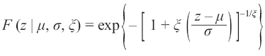
The GEV distribution arises as a limit distribution as presented by ^{Pickands (1975)} and in reference to block maxima extreme values. The GEV distribution focuses on the statistical behavior of Z_m = max {Y₁...,Y_m}, where Y ₁ , Y ₂ ..., is a sequence of independent and identically distributed random variables with common distribution function G. Here m represents the block size used to compute Z_m. A limit theorem shows that Z_m has a distribution function F that is non-degenerate and belongs to the extreme value family which includes the Gumbel, Frechet or Weibull distributions. The GEV distribution unifies the parametric representation of the three different families associated to the extreme value family as presented, for example, by ^{Coles (2001)}, ^{Reiss and Thomas (2001)}, and ^{Haan and Ferreira (2006)}. The GEV distribution has a cumulative distribution function of the following form:

(1)

for where μ is the location parameter, σ > 0 the scale parameter and ξ the shape parameter. In practice, one selects a finite value of the block size m and treats the GEV distribution as a probability model to be estimated and to represent the observed values of Z_m. This model can be assessed through plots that compare empirical versus model-based probabilities as discussed extensively in ^{Coles (2001)}. In our case, Z_m are the monthly maxima of O₃ levels per geographical zone in Mexico City as defined through Table I.

2.2 Bayesian inference

Asume we are interested on making inferences about an unknown set of parameters θ and that we have some prior beliefs about this vector, which can be expressed in terms of a prior probability density function p(θ). In addition, asume that for n observations Z = (Z₁...,Z_n) its probability distribution depends on θ and is expressed by f( Z | θ ). Bayesian inference is based on p( θ | Z ) the posterior probability distribution of θ given Z , which is computed via the Bayes theorem as

where α means "proportional to". Summaries of this probability distribution such as the mean, median or quantiles provide a few of the basic elements of statistical inference from a Bayesian perspective. In practice it is often necessary to approximate p( θ | Z ) and its summaries via numerical methods. MCMC methods offer a flexible way to deal with these high dimensional integration problems through iterative stochastic simulation algorithms that provide samples from the posterior and/or predictive distributions of interest. These samples can then be summarized in terms of histograms, sample means, medians or quantiles as illustrated in ^{Lee (1997)} and ^{Koch (2007)}. Here θ is a generic way to represent all quantities that are uncertain in a statistical model. This could consider true parameters or unobserved data points such as missing or future observations.

2.3 Statistical modeling

We assume that the monthly maximum values of O₃ per geographical zone i, Z₁,_i...,Z_T,i , are observations that follow a GEV distribution of the form

(2)

(3)

where the location parameter μ_t,i depends on β _0,i and β _1,i . β _0,i is an intercept parameter while β _1,i represents a trend in t for the location parameter and for each station; t is a time index that denotes consecutive monthly maxima values ordered chronologically, while is the mean of all the t values and sd(t) its standard deviation. Each value of t is associated to a monthly maximum zonal value that considers all the months of the years 2001-2014. It is worth noting that the grouping by geographical zone led to observations without missing values, which is a major issue in terms of model assessment when working with station level data. σ and ξ are the same for all stations and denote the scale and shape parameters of the GEV distribution as described in section 2. We also considered a version of our model that allows for σ and ξ to vary across zones and compare it to the constant model. The variability on the estimates of these parameters is very small, therefore, we decided to report results for the simpler model described in this section. We also assume that β _0,i and β _1,i are independent random quantities, also known as random effects, that follow a normal/Gaussian probability distribution and that are centered around the means m₀ and m₁ , respectively. More specifically,

(4)

where v₀ and v₁ represent the variances of β _0,i and β _1,i .

As previously described, in a Bayesian context, prior distributions are required for all model parameters. p(m ₀), p(m ₁), p(v₀), p(v₁), p(σ) and p(ξ ) denote the marginal prior distributions of m ₀, m ₁, v₀, v₁, σ and ξ , respectively. Since there is no preliminary available information on these parameters, we select locally uniform distributions with a range in (-α, α) for m ₀ and m ₁. Since σ, v₀, v₁ must be quantities greater than zero, we chose gamma and inverse gamma probability distributions centered at the value 1 and with a large variance. For the shape parameter ξ we assigned a uniform prior distribution on (-0.5, 0.5) to impose regularity properties of the maximum likelihood estimators of the GEV distribution as described by ^{Coles (2001)}. In our analyses, this prior has not a significant impact on the resulting posterior distribution of ξ and therefore in the analyses provided in this paper, one could use other priors where ξ belongs to an unbounded set.

Alternatively to a model based on a GEV distribution, we also consider a model where the observations Z _it follow a normal distribution N(μ _t,i, σ) where μ _t,i has the same structure as described in Eq. (3) and σ is a common variance across zones. For this case, μ _t,i is the mean of the observations and changes on this mean are estimated via the values β _0,i and β _1,i . The parameters β _0,i and β _1,i are also treated as Gaussian random effects.

3. Results

We sampled the joint posterior distribution defined by the model in section 2.3 using the software Open-BUGS/Winbugs as in ^{Lunn et al. (2000)}. A burn-in period of 10 000 MCMC iterations was performed, with an additional 10 000 MCMC iterations collected to produce posterior inferences. The MCMC produce samples of the posterior for all unknown quantities of our model and achieves convergence very quickly. Convergence was checked and monitored through history or trace plots and autocorrelation plots. In Figure 1 we show time series of the monthly maxima of O₃, for the years 2001-2014 and for each of the five geographical zones as defined through the stations presented in Table I. In addition, we include a zonal point estimate of the median of the GEV distribution given by the expression (see ^{Coles, 2001}). This posterior mean estimate was computed as a sample average across the MCMC simulations of β _0,i , β _1,i σ and ξ . All the median estimates are lines that have a negative slope given the model parameter structures. There is no missing information for the data shown in Figure 1. However, if one attempts to fit a similar model to the station-by-station observations of Table I, the amount of missing information is so large that our model provides very poor predictions for stations where the percentages of missing data is 50% or higher.

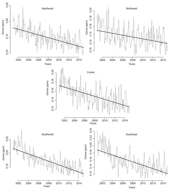
Fig 1 Monthly maxima of ozone concentrations for five geographical zones of Mexico City and estimates of μt,i(log⁡2-ξ-1)ξ given by its posterior mean. 

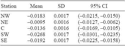
Figure 2 presents histograms of the posterior samples and density estimates of the marginal posterior distribution for β _0,i , i = 1,2,...,5 labeled by its geographical zone. The histograms are drawn by smoothing the MCMC samples with a density estimator. Table II reports posterior summaries for each β _0,i parameter where the indexes i = 1,2 denote the NW and NE zones, i = 3 represent the C zone and i = 4, 5 denote the SW and SE zones. The summaries include posterior mean estimates, posterior standard deviations and 95% credible intervals computed with the 2.5 and 97.5% quantiles. The values of β _0,i range from 0.12 to 0.16 and the posterior standard deviations are very similar across zones. The southern zones have greater estimates of β _0,i meaning that at the beginning of 2001, its location parameter had higher values. Furthermore, Figure 3 presents histograms of the posterior samples and density estimates of the marginal posterior distribution for β _1,i while Table III reports posterior mean estimates, posterior standard deviations and 95% credible intervals for these parameters. It is worth noting that β _1,i determines the rate of change in t for the median estimates of Figure 1. The posterior mean estimates have negative values in all the cases. The posterior standard deviations have almost the same values across zones. The 97.5% quantile is less than zero in all cases, therefore the credible intervals are completely contained on the negative side of the real line. The posterior distributions of Figure 3 confirm that the β _1,i parameters are essentially negative with a very high probability.

Fig. 2 Posterior distributions for β _0,i, i = 1...,5. 

Table II Posterior mean, posterior standard deviations and credible intervals for the parameter β _0,i for five geographical zones: Northwest (NW), northeast (NE), center (C), southwest (SW) and southeast (SE). 

Fig. 3 Posterior distributions for β _1,i, i = 1...,5. 

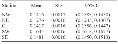
Table III Posterior mean, posterior standard deviations and credible intervals for the parameter β _1,i for five geographical zones: Northwest (NW), northeast (NE), center (C), southwest (SW), southeast (SE). 

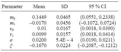
In Figure 4 we present histograms and marginal posterior densities for m ₀, m ₁, σ and ξ according to the model described in section 2.3. The histograms are drawn by smoothing the MCMC samples with a density estimator. In Table IV we report some posterior summaries for these parameters along with summaries for v₀ and v₁. The estimated variances of β _0,i and β _1,i around the values m ₀ and m ₁ are of the order of 0.01. For m ₁ its posterior probability distribution is centered at around -0.0170 with a range of values that covers negative and positive values. In particular, the posterior probability of m ₁ being less than zero given our statistical model and the data, P(m ₁ < 0|Z), is 0.6955. This value is obtained by the frequency of times in which m ₁ is less than zero over the total of 10 000 MCMC draws of m ₁. The global mean of β _1,i is negative with a moderately high probability value, although the probability interval of m ₁ includes zero. The estimated value of σ is around 0.02 and the shape parameter ξ is clearly negative which corresponds to a tail behavior of an inverse Weibull according to the extreme value distribution. Furthermore, we compare the resulting posterior estimates for m ₁ by fitting our model to the observations for years 2001-2006 and then for the observations for years 2007-2014. Our comparisons are illustrated in Figure 5 and estimates of m ₁ with credible intervals are reported in Table V. We notice that for years 2007-2014 the probability density of m ₁ is more centered around zero than the density corresponding for all years (2001-2014) and the one for 2001-2006. In fact, the mean estimate of m ₁ for 2001-2006 is -0.0168, very close to the one obtained for all years, while for 2007-2014, the mean estimate is -0.0048. The probability for m ₁ being less than zero is equal to 0.6868 for the period 2001-2006, and is equal to 0.5557 for the period 2007-2014, which essentially gives equal chance to this global parameter of being negative or positive.

Fig. 4 Histogram of posterior samples and densities for parameters m ₀, m1, σ and ξ. 

Table IV Posterior summaries for parameters m ₀, m ₁, v₀, v₁, σ and ξ. 

Fig. 5 Probability densities for parameter m ₁ for all years 2001-2014, 2001-2006 and 2007-2014. 

Table V Posterior summaries for years 2001-2014, 2001-2006, 2007-2014. 

In addition, Figures 6 and ⁷ illustrate the predictive performance of our model. We pretended that the five observations from December 2014 were missing, re-fitted the model and sampled the posterior predictive distributions for these five cases as part of our MCMC runs. In Figure 6 we show out-of-sample histograms and densities of the marginal predictive distributions by zone and for December 2014. The triangle on the x-axis represent the actual observed value. As we can see from this figure, the actual observed values are well contained within the support of the predictive distributions. In Figure 7 we show the posterior predictive mean (solid line) for each data point along with their 2.5% and 97.5% predictive limits (dashed line). The predictive means and limits are driven by the model assumptions that were made. The proposed model captures time changes in a linear fashion and provides reasonable marginal predictions. In addition, Figure 8 reports information about the μ _t,i parameters that define the trend behavior of the model. The solid lines are the values of the posterior mean estimates of each parameter, while the dashed lines define the limits of 95% credible intervals. The intervals tend to narrow at the middle of the time period of the data while the posterior mean values are lines with negative slope. Figures 7 and ⁸ clearly highlight the differences in uncertainty between prediction and parameter estimation, but lead essentially to similar point estimates of trend behavior in the data.

Fig. 6 Out of sample predictive distributions for December 2014 shown by zone. 

Fig. 7 In sample predictive means and 95% predictive intervals shown by zone. 

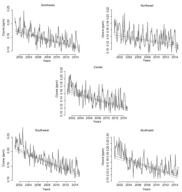
Fig. 8 Posterior means for μ _t,i, i = 1,2,...,5 represented by solid red lines and their 95% credible intervals (dashed lines) shown by zone. 

3.1 Model assessment and comparison to a Gaussian distribution model

For model comparisons we rely on the Deviance Information Criterion (DIC) as presented in, for example, ^{Banerjee (2014)}. In short, DIC is a metric that combines goodness of fit with model complexity into a numerical summary. The goodness of fit is measured through a deviance statistic that uses the log-likelihood function of the formulated model. Model complexity provides an estimate of the effective number of parameters. Alternatively, DIC can be computed as the posterior mean deviance minus the deviance at the posterior mean of the parameters. Therefore, this metric can be easily calculated via MCMC methods and can be monitored with the Openbugs software. Similar to the Akaike Information Criterion (AIC), models that achieve smaller values of DIC are considered to be better. For the O₃ monthly zonal maxima of 2001 to 2014, and the proposed model of section 2.3 based on the GEV distribution, the DIC value is equal to -4069 with an effective number of parameters equal to p_D = 11.98. On the other hand, for the model based under the assumption that the observations follow a Gaussian distribution, the DIC value is equal to -4045 with an effective number of parameters equal to p_D = 11.46. In terms of these DIC criteria, the GEV model provides a better fit to our monthly maxima data relative to a model where the observations are assumed to follow a normal distribution. We consider that DIC identifies the GEV model as a better model, since it is capable of capturing observations at the tails that a simple normal distribution may not be able to represent well. However, some of the results of our analyses under a normal model are comparable to the model based on the GEV distribution. For example, the posterior mean estimate of m₁ under the normal model is -0.01804, with a posterior standard deviation equal to 0.04566 and a 95% credible interval equal to (-0.1076,0.0700). The posterior probability that m ₁ is less than zero, P(m ₁ < 0|data) = 0.6981. For m ₀, its posterior mean is equal to 0.1537, with a standard deviation of 0.04361 and a 95% credible interval of (0.067, 0.2419).

The linearity assumption on μ is a basic assumption to represent non-stationarities in a GEV distribution framework. More general non-linear models based on the state model framework had been studied in ^{Huerta et al. (2004)} and ^{Huerta and Sanso (2007)}. Certainly these models offer an interesting alternative to the statistical models proposed in this paper. However these models are harder to estimate and require a very careful assessment of MCMC convergence. They also lack the simplicity of interpretability of the trend estimation through the m1 parameter that we offer in this paper. Furthermore, based on the posterior mean estimates of the model parameters, we considered residual probability plots for the GEV model specification as in ^{Coles (2001)} and qq-plots for the normal/Gaussian model. Figure 9 shows an example of these graphs for the observations corresponding to the NW zone. The probability plot for the GEV distribution follows closely the identity line, while the qq-plot shows some deviation from the qq-line for the largest values. The graphs for other zones are comparable and in some cases (C and SW zones) do not give any indication of lack of fit for the Gaussian model.

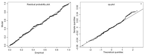
Fig. 9 Residual probability plot for GEV model (left) and qq-plot for Gaussian model (right) based on posterior mean estimates of the parameters. Northwest zone. 

We also fitted a model where both the scale and shape parameter of the GEV distribution depend on the zone, so that Y_it follows a GEV (μ_i,t, σ_i, ξ_i ) distribution where each σ _i has a gamma prior distribution and each ξ _i follows a U(-0.5, 0.5) distribution, i = 1,2,...,5. The posterior mean estimates vary from 0.018 to 0.022 while the estimates for ξ_i go from -0.13 to -0.18. On the other hand, the DIC value for this other model equals -4063 with the number of effective parameters equal to 19.04. The better model still remains to be the one where both σ_i and ξ_i are constant across the zone. However, notice that the resulting m ₁ posterior mean estimate is now equal to -0.0172 with a 95% credible interval of (-0.102, 0.07014).

4. Conclusions and other considerations

We have presented an application of the theory of extreme values in combination with Bayesian statistical modeling for a set of monthly maxima O₃ measurements derived from the RAMA network in Mexico City, and with the purpose of characterizing some of the behavior of these measurements along the years 2001-2014. Our analyses show that there is some evidence of decaying levels for these 21st century monthly maxima. We are also able to provide an overall estimate of the trend change, the m ₁ parameter, which pulls information from all the zonal data into a unique estimate along with probabilities estimates of this parameter being negative. For more recent observations corresponding to 2006-2014, the m ₁ does not provide any evidence of trend behavior for the ozone maxima.

An interesting alternative approach to the one proposed in this paper, is to treat β _0,i and β _1,i as spatial random effects rather than as pure random effects. This falls within the context of spatial areal data modeling as in ^{Banerjee (2014)}. Along with the MCMC methods, this involves the specification of a 5 x 5 adjacency matrix to define spatial associations between the five zones of interest. In a preliminary analysis of this type of modeling, for a situation where the center zone is neighbor of any other zone, the northern zones are neighbors only of each other and the center zone, and the southern zones are neighbors of each other and of the center, we found that the posterior mean estimate of m ₁ is -0.0175, with a 95% credible interval equal to (-0.019, -0.016). Other parameter estimates resulted very similar to the model that treats the parameters as random effects exclusively. The question still remains open in terms of deciding an appropriate neighborhood structure for the spatial random effects, and whether this type of models provide a more appropriate representation of the ozone maxima analyzed in this paper as compared to a pure random effects model.