Some atmospheric aerosol characteristics as determined from laser
angular scattering measurements at a continental urban station

P. ERNEST RAJ, P. C. S. DEVARA, G. PANDITHURAI,
R. S. MAHESKUMAR and K. K. DANI
Indian Institute of Tropical Meteorology, Pune - 411008, India

 

RESUMEN

Se utilizó un sistema “lidar” biestático continuo de onda de argón para obtener información sobre la variación en la intensidad de la señal láser de retorno desde la atmósfera baja con ángulos de dispersión a una altitud fija. Para el estudio se utilizaron datos lidar obtenidos en cincuenta días de cielo claro en una estación tropical urbana durante el periodo de abril de 1987 a diciembre de 1995. Los datos experimentales se compararon con las secciones transversales de dispersión de Mie obtenidas teóricamente a los ángulos comunes de dispersión para determinar el valor más probable del índice de tamaño, v, y el índice complejo de refracción, m, aplicables al ambiente sobre el sitio de observación utilizando un método de búsqueda tipo biblioteca y herramientas estadísticas simples. El estudio demostró que el aerosol que ocurre con más frecuencia es del tipo polvo y que el valor más probable del índice de tamaño es 4.5. La recuperación del número de concentración del aerosol, utilizando esta información junto con los valores experimentales de la intensidad de la señal de dispersión, dan un valor promedio de concentración de 2 - 3 x 10^-3 cm^-3en la capa atmosférica cercana a la superficie.

ABSTRACT

A bistatic continuous wave Argon ion lidar system has been used to collect information on the variation of laser return signal strength from the lower atmosphere with scattering angles at a fixed altitude of scattering. Lidar data collected on 50 clear sky days during the period of April 1987 - December 1995 at a continental tropical urban station have been used for the study. The experimental data have been compared with the theoretically computed differential Mie scattering cross sections at the common scattering angles to determine the most probable value of size index, v, and the complex index of refraction, m, applicable to the environment over the observing site by adopting a library-search method and simple statistical tools. The study showed that the most frequently occurring aerosol type at the location is dust-like with a most probable value of size index 4.5. Retrieval of aerosol number concentration, using this information together with the experimental values of scattered signal strength, yields an average concentration value in the range of  2 x 3 10³ cm^-3 in the atmos pheric layer close to the surface.

Key words: Lidar, aerosols, angular scattering

1. Introduction
Particulate material suspended in the atmosphere, commonly referred to as atmospheric aerosol, is produced by both nature and man. Naturally occurring materials include volcanic dust, meteoric dust, spores and seeds, particles of soil, sea salt, etc. Man’s activities contribute such materials as fly ash from smoke stacks, mineral particles from industrial sources, dusts from mining, particles produced from combustion, etc. With the passage of time, these aerosols are modified from their original forms by coagulation, sedimentation and other processes which tend to reduce the number of very large and very small particles, leaving particles of intermediate range ~ 0.1 - 10 μm radius in the atmosphere which have an atmospheric residence time of about one week. Particles in this size range produce significant optical effects in the atmosphere, including perturbation of the radiative transfer of energy between the sun and the earth. There is growing concern in recent years about the increased amount of aerosols in the atmosphere, especially due to various human/anthropogenic activities, and ultimately how they affect the climate on global and regional scales (IPCC, 1996). Thus, the determination of the optical properties of atmospheric aerosols has become a critical factor in assessing their climatic impact. These properties are functions of the chemical composition, concentration, morphology and size distribution of aerosols in different geographical locations, at different altitudes, etc. In their attempts to study the radiative energy exchange in the earth-atmosphere system and the effect of aerosols on this exchange, several investigators assumed aerosols as homogenous spheres so that the aerosol scattering characteristics may be uniquely and analytically determined using Mie’s solution of general scattering theory. Here the scattering coefficients are related to the size and composition of spherical particles through a size parameter and a complex refraction index.

Many practical problems associated with the scattering of laser radiation in the atmosphere require knowledge of the energy losses due to various scattering phenomena as well as that of the angular distribution and polarization of scattered radiation (Zuev, 1982). The angular variation of the intensity of light scattered from atmospheric aerosols has been studied by a few earlier investigators (Grams et al., 1974; Babenko et al., 1975; Tanaka et al., 1982; Parameswaran et al., 1984; Takamura and Sasano, 1987; Ernest Raj et al., 1995; Pandithurai et al., 1996). Laser radar (Lidar) systems have been very effectively utilized to study various aerosol characteristics because aerosols have relatively large optical scattering cross-sections (e.g., Carswell, 1983). Further, the capabilities of laser aerosol monitoring methods have been greatly enhanced with the advent of the bistatic mode of operation of the lidar, where the laser source and the receiver are separated by a finite distance, to obtain scattered intensity at various scattering angles (Reagan and Herman, 1970; Ward et al., 1973; Parameswaran et al., 1984; Ernest Raj et al., 1987). The scattered intensity from molecules varies as the cosine of the scattering angle and is governed by Rayleigh theory, while that of radiation scattered by aerosols depends on their size distribution and refractive index, governed by Mie scattering theory. A bistatic continuous wave Argon ion lidar system is in operation at the Indian Institute of Tropical Meteorology, Pune (18° 32’N, 73° 51’E, 559 m above mean sea level), India since October 1986 to obtain vertical distributions of aerosol number density in the lower troposphere. This lidar system has been used in the present study to collect information on the variation of laser-return signal strength with a scattering angle at a fixed altitude of scattering in the surface layer. This information has been used to determine the most probable values of size index, v, which represents the slope of the size distribution curve, and the refractive index, m, applicable to the observation site, by adopting a library-search (L-S) method and a simple statistical approach. The methodology followed here, the data collected and the results obtained are presented in the following sections.

2. Methodology
The bistatic lidar system at this location basically consists of a continuous-wave 4-watt (multi-line) Argon ion laser as the transmitter. The laser is operated at the prominent laser line of 0.5145 μm and the laser is linearly polarized in the vertical plane. A beam steering device is used at the transmitter-end to tilt the laser beam to the desired angle. The receiving system essentially consists of a 25 cm diameter Newtonian telescope, a narrow-band interference filter of 1 nm FWHM and a Peltier cooled photomultiplier tube. The transmitter and the receiver are separated by 60 m in the same horizontal plane. The entire lidar system is installed on the terrace of the Institute building, which is about 13 m above ground level. A detailed description of the lidar system at Pune is given in an earlier publication (Devara and Ernest Raj, 1987). The received power P_R at any scattering angle θ in the bistatic configuration is given by

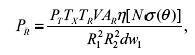
where P_r is the transmitting power of the laser and V is the volume enclosed by the intersection of the transmitting and receiving beams (scattering volume). R₁ and R₂ are the ranges of the center of scattering volume from the transmitter and receiver, and T_x and T_R are atmospheric transmittances along these paths. A_R is the collecting area of the receiver, η the system constant including the overall optical efficiencies of the system, dw₁ is the transmitted beam solid angle. N is the number density (cm^-3) of the scatterers and σ (θ ) is the differential scattering cross-section (cm² sr-¹) at scattering angle θ. Rearranging the above equation and taking all the known terms to the right-hand side, we get

N_S is subsequently referred to as normalized signal strength in the text. Now it is evident from the above equation that once the appropriate values of differential cross-section are known, from the lidar experimental data it is possible to estimate the aerosol number density within experimental error.

The scattered signal from the atmosphere contains contributions from air molecules and aerosols whose scattering cross sections differ from each other mainly because of their size differences. Thus the composite angular variation of the scattered signal depends on aerosols and molecular cross sections and the number densities, but the average scattered intensity for molecules vanishes at scattering angle 90°. Also as the probing laser wavelength in the present experiments is 0.5145 μm, the scattered intensity variations are assumed to be predominantly due to aerosols. Mie theory assumes spherical scatterers and for an aerosol unit volume having different particle radii ranging from r₁ to r₂, the differential Mie scattering cross section of aerosols, s_a (q) can be written as

where i₂ is the Mie scattering function when the incident light is polarized parallel to the scattering plane (McCartney, 1976; Chylek et al., 1975), dN_a (r) represents the number of particles between radii r and r + dr in unit volume, θ is the scattering angle, m the refractive index, r the particle size and λ is the wavelength. For computations with Mie scattering theory in the case of aerosols, the nature of the size distribution is to be known. The following modified power law distribution by McClatchey et al. (1972) has been used in the computations here.

where v is the aerosol size index (also called the Junge size exponent or the shaping parameter) and C is a normalized constant. Using the above equations, the differential Mie scattering cross sections have been computed and presented here.

3. Experimental scheme and data
The experimental schematic followed in the laser angular scattering measurements is shown in Figure 1. Scattering angle is varied from 90° to 175° in 16 steps by reorienting the transmitter and receiver elevation angles appropriately. The transmitter-receiver elevation angle combinations adopted here and the corresponding scattering angles are shown in Table 1. The Table also shows the height of the common scattering volume ( H_v ) and ranges R₁ and R₂ corresponding to the 16 scattering angles. The mean height of scattering is 30.08 m with the variation being only 0.4%. Thus, the experimental arrangement could maintain a nearly constant scattering altitude. Also, the maximum range from the lidar in the horizontal direction is about 170 m. Therefore it is fair to assume that the composition of aerosols and their number density (which are expected to vary with altitude and horizontal range) remain reasonably constant at all the above 16 scattering angles within a radius of 170 m during the experimental period of about 20 minutes. The laser angular scattering experiment is conducted generally between 1900 and 2030 hrs LT during clear sky conditions. Laser scattered signal strength (received power) from the atmosphere at all the above 16 scattering angles is recorded for a constant laser transmitter power of 200 mW. At each scattering angle, 10 to 15 values of signal-plus-noise and noise each are collected. From the mean values of received signal strength, power received is computed and at each scattering angle the normalized signal strength, N_s as given by equation (1) is computed. The angular scattering experiment is conducted once a month as part of our regular lidar measurement program. Due to unfavorable weather/sky conditions, fewer observations can be made during the monsoon season from June to September. But over the 8-year period of observations undertaken at this lidar site, the observational days were more or less evenly spread out over all the seasons and the overall average can be representative of the mean picture for this location. Thus, the data collected on 50 days during the period of April 1987 - December 1995 have been used in the present analysis.

Fig. 1.

Fig. 1. Experimental schematic for laser angular scattering measurement in the scattering
angle range 90° - 175°.

Table 1

4. Results and discussion
According to equation (1), within the limitations of experimental error, the accuracy of estimation of aerosol number density, N depends solely on the choice of the best possible values of σ_a ( θ ). Mie scattering cross-section in fact depends on scattering angle ( θ ), wavelength of probing ( λ ), size index ( v ) and refractive index ( m ). Data collected in the present study correspond to the fixed Argon ion laser wavelength of 0.5145 μm. Sixteen scattering angles used in the actual lidar angular scattering experiments and shown in Table 1 have been considered in the computations of σ_a ( θ ). In some of the earlier investigations (Parameswaran et al., 1984; Pandithurai et al., 1996) values of v considered for the computations of Mie scattering cross-sections are whole numbers like 2.0, 3.0, 4.0 etc. In the present study, 52 values of v in the range of  2.0 to 7.1 (e.g., 2.0, 2.1, 2.2, 2.3, ...., 6.9, 7.0, 7.1) have been considered to determine the closest / maximum probable value of v that can best represent the type of aerosols present over the lidar observational site. For simplicity and computational convenience, many of the investigators consider only the real part of the complex refractive index (m = 1.50) which ignores the absorption property of the aerosol under study. In the present study also this ‘no absorption’ case has been considered. Besides this, following Shettle and Fenn (1979), complex refractive index values appropriate for water-soluble (1.53 - i 0.005), dust-like (1.53 - i 0.008) and soot-type (1.75 - i 0.45) aerosols appropriate to the laser wavelength of  0.5145 μm are also considered for the analysis here.
Thus, in all four typical values of m representing different environmental conditions or those representing four different aerosol compositions are used. Now for each value of m, Mie scattering cross-section values at 16 scattering angles for each of the 52 v values (2.0 to 7.1) are computed using the equation (2). Here the upper and lower limits of integration in the equation have been taken to be 10 μm ( r₂ ) and 0.1 μm ( r₁ ), respectively. As such, the computations give 52 curves of σ_a( θ ) versus θ for each value of m. Figs. 2a - 2d show the variations of differential Mie scattering cross-sections with scattering angles for v = 2.0 to 7.1 (52 curves) for each of the above mentioned four refractive index types, namely, no absorption, water soluble, dust-like and soot-type, respectively. The digital output data from these computations is stored in the computer in readable format for comparison later with the experimental data and for further analysis by the library-search method. It may be noted from Figure 2 that the shape of the curve changes considerably for different combinations of v and m values, with minimum value of cross-section occurring between 100° and 110°. Furthermore, it is to be noted here that only 16 values of scattering angles that correspond to those used in the actual lidar angular scattering experiment are used to obtain these curves. However, if a larger number of θ values, closely spaced (within the range of 90° - 180°) were used in the Mie scattering computations, then the curves would have shown a well-defined minima and a smoother variation. Thus these 52 x 4 curves of σ_a ( θ ) have been used for comparing the experimental curve of angular variation of normalized signal strength (N_s).

Fig. 2.

Fig. 2. Variation of differential Mie scattering cross section with scattering angle for v = 2.0
to 7.1 (52 values) and for four refractive index types representing (a) no absorption,
(b) water soluble, (c) dust-like and (d) soot-type.

 

The overall mean variation of scattered signal strength (normalized signal strength, N_s) with a scattering angle in the range 90° - 175° obtained for the 50 days of observations during the period of April 1987 - December 1995 is shown plotted in Figure 3. It is seen that N_s is maximum at higher scattering angles and decreases rapidly with decreases in scattering angles of up to 105°. Then N_s increases with further decreases in scattering angles till 90°. In fact, the individual (day’s) curves of scattered signal strength versus scattering angle show that the minimum in N_s lies anywhere between 100° and 110°. The position of the observed minimum in scattered signal strength (or the shape of the curve around the minimum) gives information on the refractive index of the aerosol.

The slope of this angular distribution curve between 110° and 170° gives information on the size distribution of aerosol present in the atmosphere. It has been observed in the present data set that this slope changed from day to day. Jinhuan et al. (1985) have pointed out that there are two scattering angle regions where the volume scattering function of aerosol is very sensitive to the real part or imaginary part of the refractive index. Scattering in the range of  70° - 120° is sensitive to the real part of the complex refractive index while it is more sensitive to the imaginary part around 50°. Further, the scattering function is sensitive to both the real and imaginary refractive index parts in the range of 165° - 180°.

Fig. 3. Mean variation of scattered signal strength (normalized signal strength, N_S ) with scattering angle.

It can be seen that the shape of the observed (experimental) mean signal strength curve in Figure 3 is very similar to the theoretically computed σ_a ( θ ) curves shown in Figure 2. This is as expected, since equation (1) indicates that N_s is directly proportional to σ_a ( θ ) at constant aerosol number density, N. Now assuming that atmospheric aerosols are distributed homogeneously in the horizontal during the period of the experiment (post sunset period), the estimated aerosol number density at a constant altitude from different scattering angles should be constant or nearly equal within the limitations of experimental error. Thus, using the observed N_s values at the 16 scattering angles and choosing a particular set of σ_a ( θ ) values (i. e., for a particular combination of v and m), corresponding 16 values of N are computed using equation (1). The mean N, standard deviation and percentage coefficient of variation (% C. V.) are computed for this set of 16 values. If the above assumption of of aerosol number density at constant altitude was valid, then it is expected that the computed C. V. value would be small. Following this procedure, using the computer stored (library) values of σ_a ( θ ), percentage C. V. values are determined for a fixed value of m and for 52 different values of v from 2.0 to 7.1. The procedure is then repeated for all the four refractive index types considered in the study. Now the variation of  % C. V. with v is plotted to determine for which value of v the variability is minimum and also for which type of m it is the least. Figure 4 shows these plots on two typical days of observation, i. e., 3/14/1990 and 4/23/1992. Here the variation of  C. V. with v are shown as separate curves for different m types. It can be seen that C. V. is high for smaller values of v and it smoothly decreases with increasing v and reaches a minimum and then again it increases for higher values of v. This variation is true for all the aerosol types. The numerical value in the figure near the individual curves gives the value of v where minimum C. V. occurs for each m type. On both the days shown in Figure 4 the smallest value of  C. V. is obtained for the case of dust-like aerosols. Thus, the most probable type of aerosol on both days is dust-like, but the probable value of v is 3.8 and 4.6 respectively. A smaller value of v indicates the presence of more relatively larger- sized particles on that particular day and viceversa. Such a day-to-day variation of v can be expected as the size distribution in the surface layer in the vicinity of a large urban area can vary in source strength and transient atmospheric changes.

Fig. 4. Variation of percentage C.V. with size index v for the four different types of aerosols on two
typical days of observation

Using the mean N_s curve shown in Figure 3, the variation of % C. V. with v for different m types are obtained by the same method followed above and shown plotted in Figure 5. Thus, on an average also, it is seen that the most probable type of aerosol composition at this location is dust-type and the minimum C. V. occurred at the v value of 4.8. The value of v thus retrieved from individual days varied from 4.2 to 5.2 for the cases of ‘no absorption’, water soluble and dust-like aerosols and it varied from 2.2 to 2.9 in the case of soot-type aerosols. The frequency of occurrence of a particular v value for the 50 observation days is calculated for all the four m types and the frequency distribution histograms are shown in Figure 6. It is seen that the most frequently occurring value of v in the first three types is 4.5 and if soot-type aerosols are present over the observation site, the most probable v value then would be 2.6. The frequency distribution also shows that it is skewed more towards the larger v value side relative to the most frequently occurring value. This points out that the chances of the presence of smaller sized aerosol particles in the surface layer is greater, which again points to the influence of the anthropogenic origin of the aerosols observed over the site. The analysis further showed that 84% of the cases indicated the dominant presence of dust-like aerosols at this site. The lidar site is located on the western edge of the large urban city of Pune. There is open barren land around the site with few low-level hillocks scattered in the surroundings. About 1 km further on the western side of the site are some traditional open-air brick baking kilns and small village-like settlements. There has also been concrete building construction activity going on for several years in the area around. All these activities may be directly or indirectly responsible for the observed aerosol/particle type at the site. As the observations are close to the surface, wind blown particles may have a dominant influence. Interestingly, the soot-type aerosols were also present 12% of the time. This further points out that aerosols of urban origin like transport vehicular emissions, bio-mass burning, etc. are also showing their influence in modifying the refractive index and size distribution of aerosols in the surface layer over the lidar site. As the experimental days are more or less uniformly spread out during all the seasons of the year, the most probable size index value, v (4.5) and refractive index, m (1.53 - i0.008) can be employed with greater confidence while computing the differential Mie scattering cross sections, σ_a ( θ ) which are ultimately used in the retrieval of vertical distributions of aerosol number density with the Argon ion lidar data collected at this location.

Fig. 5. Variation of percentage C.V. with size index v for the four different types of aerosols for the
overal mean experiment data.

 

Fig. 6. Frequency distribution of estimated size index v for the four types of aerosols.

Figure 7 shows the variation of mean aerosol number density with size index for the four types of refractive indices. As expected, aerosol number concentration would be higher for a choice of a larger value of v. Thus, for a most probable value of 4.5 of v determined in the present analysis, the aerosol number density in the surface layer (at 30 m) would be in the range of  2 x 10³ to 3 x 10³ cm^-3. It is also seen that for a variation of v from 2.0 to 7.0, the estimated concentration can vary by more than 2 orders of magnitude. Therefore, for a good estimation of aerosol number density, it is essential to determine the most appropriate values of v and m, which in turn can be used to theoretically compute the differential Mie scattering cross sections. Grams et al. (1974) measured angular scattering intensities with a polar nephelometer in the range of 10° - 170° and retrieved the refractive index value, but they reported an uncertainty factor. So, Jinhuan et al. (1985) first identified the scattering angle regions where volume scattering function is sensitive to real part and imaginary part of the refractive index and then using this information found more satisfactory results while retrieving the refractive index from remote sensing methods. The experimental scheme followed in the present study and the library search method adopted in retrieving the size index and refractive index seem to yield a fair estimate of these parameters, which in turn, facilitate the inversion of lidar data.

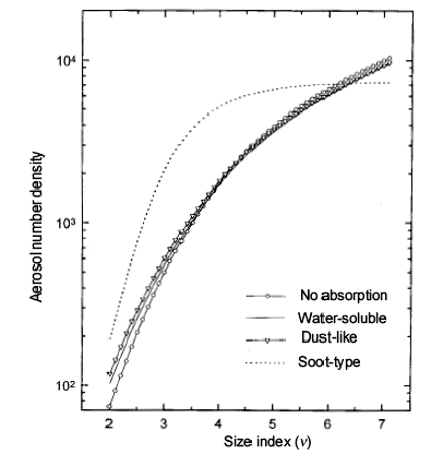
Fig. 7. Variation of estimated mean aerosol number concentration with size index v for the four
types of refractive indices.

5. Conclusions
The present study shows one of the unique advantages of operating a lidar system in the bistatic mode, where angular variation of light intensity scattered from atmospheric aerosols can be recorded. An experiment designed to make observations of scattered intensity at different scattering angles but from a constant altitude of scattering, adopting a bistatic Argon ion lidar system has been described. A simple library-search method has been used to estimate the most probable size index and refractive index values that are necessary to compute Mie scattering cross sections applicable to the observation site. This in turn will help to better estimates aerosol number density from lidar vertical profiles of scattered signal strength.

Acknowledgements
The authors would like to thank the Director, IITM for his constant encouragement. The assistance from Dr. S. Sharma in the collection of the data is gratefully acknowledged.

References
Babenko, V. A., A. P. Prishivalco and S. T. Leyko, 1975. Angular characteristics of light scattering by radially inhomogeneous particles of atmospheric aerosol particles. Atmos. and Oceanic Phys., 11, 398-400.        [ Links ]

Carswell, A. I., 1983. Lidar measurements of the atmosphere. Canadian J. Phys., 61, 378-395.        [ Links ]

Chylek, P., G. W. Grams, G. A. Smith and P. B. Russell, 1975. J. Appl. Meteorol., 14, 380.        [ Links ]

Devara, P. C. S. and P. Ernest Raj, 1987. A bistatic lidar for aerosol studies. IETE Tech. Rev., 4, 412-415.        [ Links ]

Ernest Raj, P. and P. C. S. Devara, 1989. Some results of lidar aerosol measurements and their relationship with meteorological parameters. Atmos. Environ., 23, 831-838.        [ Links ]

Ernest Raj, P. and P. C. S. Devara, 1995. Scattering angle distribution of laser-return signal strength in the lower atmosphere. J. Aerosol Sci., 26, 51-59.        [ Links ]

Grams, G. W., I. H. Blifford, D. A. Gillette and P. B. Russell, 1974. Complex index of refraction of airborne soil particles. J. Appl. Meteorol., 13, 459-471.        [ Links ]

IPCC, 1996. Climate Change 1995: The Science of Climate Change, J. T. Houghton, M. Filho, L. G. Callander, N. Harris, A. Kattenberg and K. Maskell (eds.), Cambridge University Press, New York.        [ Links ]

Jinhuan Qui, Zhou Xiuji and Zhao Yanzeng, 1985. Theoretical analysis of remote sensing of aerosol refractive index by angular scattering method. Scientia Sinica (Series B), 28, 745-757.         [ Links ]

McCartney, E. J., 1976. Optics of the Atmosphere: Scattering by Molecules and Particles. Wiley, New York.        [ Links ]

McClatchey, R. A., R. W. Fenn, J. E. A. Selby, F. E. Volz and J. S. Garing, 1972. Optical Properties of the Atmosphere (third edition), AFCRL-72-0497, AD753075, Air Force Cambridge Research Laboratories, Bedford.        [ Links ]

Pandithurai G., P. C. S. Devara, P. Ernest Raj and S. Sharma, 1996. Aerosol size distribution and refractive index from bistatic lidar angular scattering measurements in the surface layer. Remote Sensing Environ., 56, 87-96.        [ Links ]

Parameswaran, K., K. O. Rose and B. V. Krishna Murthy, 1984. Aerosol characteristics from bistatic lidar observations. J. Geophys. Res., 89, 2541-2552.        [ Links ]

Reagan, J. A. and B. M. Herman, 1970. Proc. 14^th Conf. Radar Meteorol., p.275.        [ Links ]

Shettle, E. P. and R. W. Fenn, 1979. Models for the aerosols of the lower atmosphere and the effects of humidity variations on their optical properties. AFGL-TR-79-0214, Air Force Geophysics Laboratory, Hanscom.        [ Links ]

Takamura, T. and Y. Sasano, 1987. Ratio of aerosol backscatter to extinction coefficients as determined from angular scattering measurements for use in atmospheric lidar applications. Optical and Quantum Electr., 19, 293-302.        [ Links ]

Tanaka, M., T. Nakajima and T. Takamura, 1982. Simultaneous determination of complex refractive index and size distribution of airborne and water-suspended particles from light scattering measurements. J. Meteorol. Soc. Japan, 60, 1259-1272.        [ Links ]

Ward, G., K. M. Kushing, R. D. McPeters and A. E. Green, 1973. Atmospheric aerosol index of refraction and size-altitude distribution from bistatic laser scattering and solar aureole measurements. Appl. Opt., 12, 2585-2592.        [ Links ]

Zuev, V. E., 1982. Laser Beams in the Atmosphere, Plenum, New York.        [ Links ]