1. Introduction

There exist various Milky Way models aimed at presenting the mass distribution in which the potential is given analytically. In such models it is usually assumed that there are three main contributors to the mass of the Milky Way: the bulge, the disk and the subsystem composed of the dark matter. The mass distribution in each of the three subsystems is assumed to be stationary and axially symmetric. The bulge is known to be weakly flattened, the dark subsystem has been usually regarded also as weakly flattened, so for both spherical symmetry a special case of the axial one has been applicable. In the case of the disk the spherical symmetry assumption is not acceptable for clear reasons. One should have found a suitable and sufficiently simple expression for the disk contribution to the potential. As well known examples the cases of ^{Allen and Martos (1986)} and ^{Allen and Santillan (1991)} may be mentioned. In the former paper the rather cumbersome Ollongren polynomials are used, with which there were some difficulties (^{Allen & Santillan 1991}), whereas in the latter paper the authors use the ^{Miyamoto-Nagai formula (1975)}. This formula has been used rather often for the purpose of providing the potential of the disk analytically (e.g. ^{Ninković 1992}, ^{Dinescu et al. 1999}). However, the present author (^{Ninković 2015}) has indicated that when applying the Miyamoto-Nagai formula to an exponential disk the total mass in the Miyamoto-Nagai formula and the total mass of the exponential disk are not equal. In this way it can be understood why in the Milky Way models where the disk is described by the Miyamoto-Nagai formula the total mass is unusually high, about 1.6 times higher than the value normally expected (e.g. ^{Ninković 1992}, ^{Dinescu et al. 1999}). For the purpose of describing a single subsystem, it is also possible to use a potential consisting of several terms, where each term is represented by means of the Miyamoto-Nagai formula (e.g. ^{Miyamoto and Nagai 1975}); terms with negative mass have been also introduced (e.g. ^{Smith et al. 2015}). Even then the total mass in the potential formula has not been always equal to the total mass of the system (subsystem) to which the formula is applied (e.g. MilkyWay thin disk in ^{Smith et al. 2015}).

In the present paper a new formula for the gravitational potential is proposed, which is based on the Miyamoto-Nagai formula. One of its parameters is the total mass. When this formula is applied to a stellar system (subsystem), its total mass is required to be equal to the total mass of the system (subsystem). This is the same principle as used in the earlier paper (^{Ninković 2015}), but the formalism is different.

The next sections of the present paper are organized in the following way: § 2, entitled Description, contains the formulae necessary for further work. § 3, Rotation Curve, is devoted to the resulting rotation curve(s). § 4, Density, deals with the density corresponding to the potential proposed in § 2. In § 5 Application to the Milky Way Disk, there is a discussion concerning the consequences for the Milky Way. Finally Discussion and Conclusion are presented in § 6 and § 7. Since the main text contains the most important formulae only, it is followed by an Appendix, in which all relevant formulae are given.

2. Description

As is well known, the potential formula of Miyamoto and Nagai has the following form:

where G is the universal gravitation constant and M the total mass of the system (subsystem) generating the gravitation field; a and b are two constants with dimension of length, whereas R and z are the variables on which the potential Φ depends. The potential given by formula (1) is stationary, because it does not depend on time explicitly, and axially symmetric, because it is independent of the third coordinate in a cylindrical system (the angle).

The extreme cases are: α = 0 and b = 0. Both were already known at the time the Miyamoto-Nagai formula was published. All the relevant details can be found in the paper of ^{Miyamoto and Nagai (1975)}. Here it will be only briefly said that α = 0 corresponds to spherical symmetry; otherwise the source system is flattened. In the extreme case of flattening (b = 0) the density is infinite in the midplane (z = 0), outside it is equal to zero.

The term in the denominator of equation (1), as introduced by ^{Miyamoto and Nagai (1975)}, will be referred to as the Miyamoto-Nagai (MN) function. It has the dimension of length; the expression is given in the Appendix (equation A14).

According to the modification proposed in the present paper there will be two MN functions F₁ and F₂, which will differ in their constants (F_i with a_i and b_i, i = 1, 2). The potential will be given then as:

where the constant term GM has the same meaning as in (1).

In what follows an analysis of the modification (2) will be presented. In the first step the resulting rotation curve will be the subject, in the second one the density.

3. Rotation curve

Usually the term “rotation curve” refers to the circular speed. The circular speed u_c is defined through the first partial derivative of the potential with respect to R. Except the special case of spherical symmetry (the constants in equation 2 have values α_i = 0), when circular motion can occur in any plane containing the center (R = 0, z = 0), in the more general case (α_i≠ 0) circular motion can take place only in the midplane z = 0. With regard to equation (2) the circular speed will be given in the following way:

In (3) Φ is the potential (equation 2), and it takes into account that the first partial derivative of F_i in R is equal to R/F_i (Appendix equation A15). Since z is zero, in either MN function the parameters α_i and b_i participate only through their sum. In other words the ratio b_i/α _i is of no importance for the behavior of the circular speed. Its behavior will be the same, including the simplest case α_i = 0 (i = 1, 2, spherical symmetry). In the case of spherical symmetry one can use the cumulative mass Mr (r=R2+z2). The expression for the cumulative mass is similar to that for the circular speed (3), it is

Since now both F_i (i = 1, 2) have the simpler form bi2+r2, the expression within brackets in (4) can be presented less generally. It takes the following form:

Expression 5 is important because the cumulative mass must not be negative. The immediate consequence is that b₁/b₂ should exceedαα+1. The same is valid for the circular speed (equation 3), but since then α _i can be different from zero, the condition should be rewritten to become

The circular-speed value, being zero for R = 0, increases afterwards to attain a maximum. The distance R = R _m at which the maximum occurs depends on α and on the ratio (α₁ + b₁)/(α₂ + b₂). In general, when this ratio approaches its critical value (equation 6), the maximum R_m occurs farthest from the center. How far it lies depends on α. The smaller α, the smaller the value of R_m expressed in terms of α₂ + b₂. As the ratio (α₁ + b₁)/(α₂ + b₂) increases, the maximum is shifted towards the center. In this way, for a given α there exists an interval for the maximum on the rotation curve expressed in terms of a₂ + b₂. The interval width depends on α. The smaller α, the narrower the interval. Finally, when α tends to zero, the interval width also tends to zero. This is understandable because α = 0 corresponds to the Miyamoto-Nagai case where, as is well known, the maximum on the rotation curve occurs at Rm=2a+b. When α tends to infinity, the lower limit of the interval (corresponding to (α₁ + b₁)/(α₂ + b₂) infinitely large) tends to zero, whereas the upper limit is about 2(α₂ +b₂). The upper limit corresponds to the lower limit for the ratio (α₁ + b₁)/(α₂ + b₂) (equation 6), which for very high α is practically equal to one.

Formula (1) has been frequently used as a suitable approximation for an exponential disk (e.g. ^{Ninković 1992}). The rotation curve of the exponential disk was calculated by ^{Freeman (1970)}. In his paper a plot of circular speed versus distance in the midplane is given. It is interesting to compare the circular speed obtained here (equation 3) with the curve obtained by ^{Freeman (1970)}. The comparison is given in Figure 1. Since the units for R (abscissa) and u_c (ordinate) must be the same for both curves, the curve obtained on the basis of (3) also corresponds to the exponential-disk scale R _d along the axis of abscissae and to GMRd along the ordinate axis. Here the total mass M is the same as that of the exponential disk, whereas the ratio (α₂ + b₂)/R _d should be established from the comparison. The ratio (α₁ + b₁)/(α₂ + b₂) is established simultaneously. Both ratios depend on α. The two curves are required to have a common point at the maximum (Figure 1), hence the same R _m and u_c(R _m). Such a fit can be achieved for any α. However, when α tends to zero, the ratio (α₂ + b₂)/R_d tends to about 1.5, whereas (α₁ + b₁)/(α₂ + b₂) tends to infinity. On the other hand, when α tends to infinity, the ratio (α₂ + b₂)/R_d exceeds two and the ratio ((α₁ + b₁)/(a₂ + b₂)) tends to unity. Thus any satisfactory fit (corresponding to a particular value of α) of the rotation curve on the basis of (3) to the curve presented in ^{Freeman’s (1970)} paper is obtained if both (a₂ + b₂)/R_d and (α₁ + b₁)/(α₂ + b₂) are greater than 1. In the case of the former ratio this can be expected, since the fitting of the curve given by Freeman (1970) by the model based on equation (1) yields a + b of about 1.5R_d. As for the latter ratio [(α₁ + b₁)/(α₂ + b₂)], it can be said that the values yielded by the fits, for α ≥ 1.5, are approximately equal to [(α + 1)/α]^0.8.

Fig. 1 Rotation curve u_c (R)(u_c unit isGMRd, black thick line from ^{Freeman (1970)}, dashed curve, Keplerian curve for the same mass, also taken from Freeman’s paper, green line as obtained here, α = 1, a₂ + b₂ = 2.04R_d, α₁ + b₁ = 3.7R _d, blue line from ^{Ninković 2015} (parameter values -α +b = 2.1R _d, Υ1=-0.1, their meaning look for in equation (7) of that paper), red line according to expression (1),a+b 2.12Rd; all curves are for the same total mass M. The color figure can be viewed online. 

4. Density

Now the density generating the potential given by (2) will be calculated. As is well known, the density ρ is related to the potential Φ through the Poisson equation

In equation (7) the axial symmetry is taken into account, i.e. the angle term is omitted because the potential is independent of this coordinate. The relevant expressions for the potential derivatives can be found in the Appendix.

It has been already mentioned (§ 3) that the ratio (α₁ + b₁)/(α₂ + b₂) should obey condition (6); otherwise in the central parts the density will be negative. In such cases the density increases in the central parts to attain zero, then it continues to increase so that its maximum occurs away from the center. This trend persists even when condition (6) is fulfilled. If the highest density is required just at the center, then the lower limit for the ratio (α₁ +b₁)/(α₂ +b₂) as specified by (6) is too small. A larger value of this ratio is needed. Only then, the density will be not only everywhere non-negative, but its highest value will occur just at the center, and it will be lower at any other position. For instance, let α = 1, α₁ = α₂ = 0 (spherical symmetry), then the density will satisfy both conditions (to be everywhere non-negative and to attain its highest value at the center) only if the ratio b₁/b₂ exceeds about 0.85. Therefore, this value (about 0.85) appears as an effective lower limit for the ratio b₁/b₂, though the value following from (6) is smaller (about 0.71).

Nevertheless, in the literature there exist models with a central hole (e.g. ^{Einasto & Haud 1989}), in which the density is equal to zero at the center. Bearing this in mind the example mentioned in the preceding paragraph (b₁/b₂ ratio as low as2-1 for α = 1) can be meaningful.

The examination of the simplest case of spherical symmetry (α₁ = α₂ = 0) allows one to establish an upper limit for the ratio (b₁/b₂). If this ratio exceeds α+1α, then the density will have negative values in the periphery. More precisely, the cumulative mass (expression 4) will attain a maximum, after which it will begin to decrease.

The ratio (α₁ + b₁)/(α₂ + b₂) for given α is determined through fitting an assumed rotation curve. Unlike the special case of spherical symmetry, when one has α₁=α₂=0, in the general case the ratios b₁/α₁ and b₂/α₂ may differ, but one cannot expect solutions with physical meaning, such as, for instance, b₁ ≈ 0, α₂ ≈ 0. If extremely flattened systems (subsystems) are the subject, then it is clear that necessarily α_i ≫ b_i, i = 1,2. If it is also required that the density decrease monotonously and that its highest value occur at the center, then generally it may be accepted that b₁/α₁ = b₂/α₂. These ratios may be subjected to further variations, to assume finally different values, but this would be only an adjustment.

When significantly flattened systems (subsystems) are under study, then the density decreases very rapidly off the plane z = 0, to attain zero at a finite distance from that plane. Beyond this distance it is difficult to obtain the density values everywhere equal to zero by using an analytical potential with algebraic functions developed for the purpose of finding a suitable approximation. Therefore, negative density values are inevitable, but their moduli are very low (Figure 2). In the plane z = 0 negative densities are also possible, but it is easier to avoid them. The optional parameter α is influential here; by increasing its value it is possible to shift upwards the distance from z = 0 where the density attains zero. The complete removal of negative densities can take place in infinity only, α → ∞.

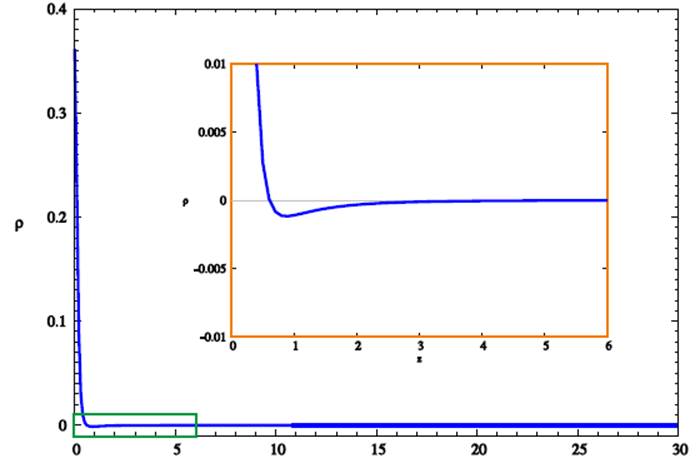
Fig. 2 Density dependence on z for R = 0; α = 1, b_i /α_i = 0.105, (α₁ + b₁)/(α₂ + b₂) = 3.7/2.04 (see Figure 1). The units are: Rd and M/R_d ³ 

The isodensity surfaces for positive density values are disky, i.e. they are inside the equivalent spheroid (Figure 3). This is the same situation as for the classical Miyamoto-Nagai model.

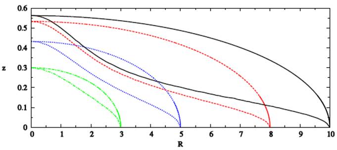
Fig. 3 Projected isodensity surfaces; each of them is presented with its comparison spheroid (the same color); α = 1, b_i/α_i = 0.105, (α₁ + b₁)/(α₂ + b₂) = 3.7/2.04 (see Figure 1). The color figure can be viewed online. 

5. Application to the milky way disk

Since the exponential disk is known to follow generally the decreasing trend of the volume density (e.g. ^{Cuddeford 1993}), then in the application of (2) it will be required that b₁/α₁ = b₂/α₂. An example may be the application to the disk of the Milky Way. The following values are assumed: M_d = 5.1 × 10¹⁰ M_⊙ for the total mass, R_⊙ = 8.5 kpc and R_d = 2.8 kpc. This mass value is substituted in equation 2, i.e. (3). The parameter α is optional; let it be α = 1. Then one will have α₂+b₂ =2.04R_d =5.7 kpc, α₁+b₁=3.7R_d=10.4kpc. The values of the factors, 3.7 and 2.04, come from the fit presented in Figure 1 (green line), which corresponds to α = 1. Now using equations 2 and 3 one can calculate the circular speed for any value of R (distance to the rotation axis). For instance, at R = 5.7 kpc and R = 8.5 kpc the circular speed will be equal to 179.5 km s⁻¹ and 169.7 km s⁻¹, respectively. The former value is practically the one where the circular speed maximum is expected. If the classical Miyamoto-Nagai formula (equation 1 in the present paper) were applied, but with the same total mass, the corresponding results would be: u_c(5.7) = 145.7 km s⁻¹, u (8.5) = 139.9 km s⁻¹. In this case α + b (equation 1) must be2 times smaller than the distance at which the circular speed is maximal. As already said, the only way out, if using equation 1, is to substitute for the total mass another value, which exceeds the assumed one (5.1 × 10¹⁰ M_⊙). This is clearly shown in Figure 1.

If accepted, the value of about 170 km s⁻¹ obtained in the preceding paragraph (provided that the circular speed at the Sun is 220 km s⁻¹) will result in a disk contribution to the square of the circular speed of about 60%. Any discussion of this value involves many factors both qualitative and quantitative. More precisely, one should identify the other subsystems and estimate the fraction of each subsystem. In addition, the dependence on R of the fractions of other subsystems can be useful, because then it will be possible to estimate the gradient or, as usually done, the ratio A/|B| (A and B are the Oort constants). As a very preliminary result it may be concluded that a disk fraction of about 60% would yield an A/|B| ratio equal to 1.0 or slightly exceeding 1.0.

Since it is required that b₁ /α₁ = b₂ /α₂, and the sums α₁ + b₁ and α₂ + b₂ are already known, we still have to determine the values of b_i. This will be done by requiring the density at R = R _⊙, z = 0 to be equal to 0.08 M _⊙ pc⁻³. The formulae given in the Appendix then enable us to determine the ratios b_i/αi, i.e. a_i, b_i; one obtains: α₁ = 9.5 kpc, b₁ =0.9 kpc,α₂ =5.2 kpc,b₂ =0.5 kpc.

6. Discussion

In Figure 1 there is also a curve corresponding to the formula proposed in ^{Ninković 2015}. As can be expected, the two formulae (the one proposed here, equation 2 and that from ^{Ninković 2015}) yield almost identical values for the circular speed for the same total mass and scale of the disk. However, these formulae are intrinsically different. Unlike the present one, wherein one has a fraction with two Miyamoto-Nagai terms, the potential formula from ^{Ninković 2015} contains an additional term in the denominator. This term is a sum of two functions, each one a single-argument function (R or z), and it is subtracted from the Miyamoto-Nagai term; the numerator contains the product GM only. For the rotation curve only the term depending on R is of importance. Its form is:

This term is added to the function f₂(z) of analogous form (f₂(z) equal to 1 in midplane) and the sum is multiplied by12R _d. The exponent γ₁ must 2 be less than 0.5. The best fits are achieved when it is slightly less than zero (-0.1, -0.3, as written in ^{Ninković 2015}). The meaning of the additional term in the denominator is that f₁(R) and f₂(z) are corrective functions, which should improve the fit. In principle, a satisfactory fit might be achieved if both f₁(R) and f₂(z) were equal to 1, i.e. if the constant R_d were subtracted from the Miyamoto-Nagai term in the denominator and if it were assumed that α + b = 2R_d. It is important to mention that the potential formula proposed in ^{Ninković (2015)} has a limited use, i.e. it is applicable to flattened systems, as indicated in the title of the paper. The only common characteristic is the following principle: if either of the two formulae is applied to a stellar system (subsystem), then the total mass of the system (subsystem) is substituted in the formula, as was done in the example of the preceding section. The total number of parameters is six in both cases: M, α, b, R _d, γ₁ and γ₂ (^{Ninković 2015}), i.e. M, α, α₁ , b₁ , α₂ and b₂ (here). However, as already said, these parameters are not completely independent. In the former case the number of parameters is, practically, reduced to three (M, α, b). In the latter case it would be also three (M, α₁, b₁), but provided that b ₁/α ₁ = b ₂/α ₂. In principle, this equality is acceptable, but not obligatory. As said above, there is a possibility of further varying either of the two ratios b₁/α₁ and b₂/α₂. This can be an advantage for the approach proposed here in comparison to that presented in ^{Ninković 2015}. The comparison concerns flattened systems (subsystems) only. If weakly flattened ones are taken into account, there is no comparison, the present approach is the only one acceptable.

In the application of potential (2) to the disk of the Milky Way at first one specifies the optional parameter α and assumes values for the disk total mass and scale length. Then the rotation curve fit, as presented in Figure 1 for the case α = 1 (green curve), yields the two sums α¹ + b ¹ and α² + b² expressed in terms of the disk scale length. Taking into account the mass assumed for the disk (provided that the circular speed at the Sun is known) it is possible to calculate the contribution of the disk to the square of the local circular speed and to give a preliminary estimate for the ratio A/|B| (A and B are the Oort constants). For reasonable values of, say, 5.1 × 10¹⁰M_⊙, 2.8 kpc and 220 km s⁻¹ the disk fraction to the circular speed squared would be about 60% and the ratio A/|B| would be about 1 or slightly larger. The ratios b_i/α_i , if put equal to each other, can be determined after assuming a value for the disk density at the Sun. For instance, if 0.08 M_⊙ pc⁻³ is assumed, b_i/α_i will be about 0.095.

7. Conclusion

In the present paper a formula (equation 2) is proposed, which serves for the purpose of calculating the gravitational potential of a stellar system (subsystem) for the case of steady state and axial symmetry, provided that the mass of the system (subsystem) is equal to the mass in (2). It has the following properties: