SciELO - Scientific Electronic Library Online

 
vol.68 issue6The q-deformed heat equation and q-deformed diffusion equation with q-translation symmetryRelativistic hyperbolic motion and its higher order kinematic quantities author indexsubject indexsearch form
Home Pagealphabetic serial listing  

Services on Demand

Journal

Article

Indicators

Related links

  • Have no similar articlesSimilars in SciELO

Share


Revista mexicana de física

Print version ISSN 0035-001X

Rev. mex. fis. vol.68 n.6 México Nov./Dec. 2022  Epub July 31, 2023

https://doi.org/10.31349/revmexfis.68.060701 

Research

Gravitation, Mathematical Physics and Field Theory

Radiation from a dipole perpendicular to the interface between two planar semi-infinite magnetoelectric media

O. J. Francaa  * 

L. F. Urrutiab  ** 

a Institut für Physik, Universität Kassel, Heinrich-Plett-Straße 40, 34132 Kassel, Germany. Instituto de Ciencias Nucleares, Universidad Nacional Autónoma de México, 04510 México, Ciudad de México.

b Instituto de Ciencias Nucleares, Universidad Nacional Autónoma de México, 04510 México, Ciudad de México.


Abstract

We consider two semi-infinite magnetoelectric media with constant dielectric permittivity separated by a planar interface, whose electromagnetic response is described by non-dynamical axion electrodynamics and investigate the radiation of a point-like electric dipole located perpendicularly to the interface. We start from the exact Green’s function for the electromagnetic potential, whose far-field approximation is obtained using a modified steepest descent approximation. We compute the angular distribution of the radiation and the total radiated power finding different interference patterns, depending on the relative position dipole-observer, and polarization mixing effects which are all absent in the standard dipole radiation. They are a manifestation of the magnetoelectric effect induced by axion electrodynamics. We illustrate our findings with some numerical estimations employing realistic media as well as some hypothetical choices in order to illuminate the effects of the magnetoelectric coupling which is usually very small.

Keywords: Magnetoelectric effect; dipole radiation; electromagnetic wave propagation

1 Introduction

The radiation produced by an electric dipole near a planar interface has been well studied over the years and has remained a relevant subject of research for physicists and engineers due its relevance in a wide range of phenomena like practical applications in radio communications [1], THz Zenneck wave propagation [2], near-field optics [3], plasmonics [4] and nanophotonics [5], just to mention a few examples. In 1909, Sommerfeld [6] published a theory for a radiating vertically oriented dipole above a planar and lossy ground which formed the basis for subsequent investigations [7,8,9,10,11]. Probably, by the fact that the early theory of dipole emission near planar interfaces was written in German, although there was an English version summarized in Sommerfeld’s lectures on theoretical physics [12], many aspects of the theory were reinvented and clarified over the years [13,14,15,16].

Here we consider planar interfaces constructed with linear homogeneous and isotropic magnetoelectric (ME) media giving rise to the so called magnetoelectric effect (MEE), whereby electric (magnetic) fields are able to induce additional magnetization (polarization) in the material. This effect, which was predicted [17] and discovered [18] in antiferromagnets, has been widely studied along the years in multiferroic materials and it is codified in an additional parameter of the material: the magnetoelectric polarizability (MEP) [19]. The recent discovery of three-dimensional topological insulators (TIs) has boosted the interest in this topic by providing new materials where this effect is predicted to occur [20,21,22,23,24,25]. Generally speaking, TIs belong to a novel state of matter in which the characterization of their quantum states does not fit into the standard paradigm of condensed matter physics whereby the phases of the material are classified according to order parameters arising from the spontaneous symmetry breaking of the corresponding Hamiltonian according to the phenomenological Ginzburg-Landau theory. A distinguished example of this classification are normal superconductors, where gauge invariance is spontaneously broken. Instead, these states are classified according to topological invariants that arise in the Hilbert space generated by the corresponding Hamiltonians in the reciprocal space of the crystal lattice. They are protected by time-reversal-symmetry (TRS) and admit an insulating bulk together with conducting surface (edge) states. The imposition of this symmetry yields two classes of materials: standard insulators labeled by a zero MEP and TIs characterized by a MEP equal to π. These new materials host a number of exceptional electromagnetic properties. Among them we have: (i) they can carry currents along the edge channels without dissipation, (ii) their MEP is quantized, (iii) the conducting edge states can be interpreted as quasi-particles being massless Dirac fermions. This by itself is an important feature that makes contact with high energy physics and which provides the opportunity to investigate the existence of unseen particles like Majorana fermions, for example. (iv) they are predicted to exhibit the quantized photogalvanic effect in which light can induce a quantized current. For an extensive review of the properties of TIs see for example [26,27,28]. All these new features provide additional motivation to reconsider the problem of radiation in magnetolectric media.

The effective theoretical framework to deal with magnetoelectric media is motivated by axion electrodynamics [29], which consists of adding the term La=gaγγ a(t,x)FμνF~μν to the Maxwell Lagrangian density Lem, plus a kinetic and a mass terms for the pseudoscalar field a(t, x). The so called axion field a(t, x) was introduced in Ref. [30] to propose a solution for the strong CP problem in strong interactions [31,32]. In the original formulation [29], the coupling constant gaγγ arised from a specific grand unification model of the strong and electroweak interactions. Also, Fμν is the electromagnetic tensor and F~μν=(1/2)ϵμναβFαβ is the dual tensor. The well known relation FμνF~μν=-4 EB allows to rewrite La in terms of the electric E and magnetic B fields. As we will show in the following the coupling La encapsulates the MEE which characterizes the electromagnetic response of the materials we consider in this work. Thus we restrict ourselves to a non-dynamical axion field a(t,x)ϑ(x), to be called the magnetoelectric polarizability (MEP), which we consider as an additional electromagnetic property of the medium, in the same footing as its permittivity and permeability [23,33,34]. Following a standard convention we now consider the interaction term Lϑ=-(α/4π2) ϑ(x)EB, where α is the fine structure constant characteristic of the electromagnetic interaction between fermions and photons in the material, which produces this effective term. We call ϑ-Electrodynamics (ϑ-ED) this restriction of axion electrodynamics and our purpose is to study the radiation produced by a dipole oriented vertically with respect to the interface between two semi-infinite planar magnetoelectric media, having different constant MEPs. Excluding important differences in their microscopic structure, we will refer to the medium as a magnetoelectric, or a ϑ-medium, as long as its macroscopic electromagnetic response can be described in the framework of the ϑ-ED.

The paper is organized as follows. In Sec. 2, we present a review of ϑ-ED which also contains a summary of the calculation of the time-dependent Green’s function (GF) for the 4-potential Aμ in our setup. As the source of the electromagnetic fields, in Sec. 3 we introduce an oscillating vertically oriented point-like electric dipole located at a distance z0 > 0, on the z-axis perpendicular to the interface between the two media. The convolution of this source with the GF is carried out in the Subsec. 3.1 and yields the corresponding electromagnetic potentials Aμ in terms of closed integrals which are calculated in the Appendix A. The next step is to obtain the far-field approximation of those integrals. This is performed using a modified version of the steepest descent method, which is appropriate to the situation where the integrand is not a smooth function in the vicinity of the stationary phase due to the appearance of poles in the steepest descent path at this point.

This approximation,which heavily relies upon Ref. [13] is explained in detail and carefully carried out in the Appendix B. These results are summarized in the Subsec. 3.1.

As a consequence of the presence of the pole we find that the 4-potential acquires a contribution from axially symmetric cylindrical waves (denoted also as surface waves) besides the standard spherically symmetric ones. A detailed analysis on the former kind of waves allows us to introduce what we call the discarding angle θ0, which permits us to divide the space in two regions: V1 where the cylindrical wave contribution can be neglected and V2 where this contribution has to be considered within a certain range of parameters in what is called the intermediate zone in the literature [13]. To characterize the relevance of these cylindrical waves we introduce a rapidly decreasing function measuring their amplitude and realize that for observation distances further away from the intermediate zone in the region V2 they turn out to be very much suppressed with respect to the spherical ones. This situation is quantitatively explained in detail also in the Subsec. 3.1. In Subsec. 3.2, the far-field expressions for E and B are calculated for each region. In Sec. 4 we consider the angular distribution, the total radiated power and the energy transport of the dipolar radiation. In the Subsec. 4.1 we establish the numerical parameters to be used in the subsequent applications. Subsection 4.2 comprises a detailed examination of the angular distribution spectrum dP/dΩ in the region V1. In Subsec. 4.3, we calculate the power radiated into the region V1. Subsection 4.4 is devoted to the energy transport of the radiation in the region V2. Here we also give some numerical estimations considering the media already discussed in Subsecs. 4.2 and 4.3, plus some additional hypothetical choices. Finally, Sec. 5 provides a concluding summary and the conclusions from our results. In the Appendix A we derive the exact expressions for the potential Aμ required to calculate the electromagnetic fields. The far-field approximation is carried out in the Appendix B using a modified steepest descent method. The final Appendix C includes a brief review of the Faddeeva plasma dispersion function which arises in the discussion of the cylindrical waves. Throughout this paper we use Gaussian units with =c=1, the metric signature is (+,—, —, —,) and ε0123 = 1. We follow the conventions of Ref. [35].

2 ϑ-Electrodynamics

Let us consider two semi-infinite ϑ-media separated by a planar interface located at z = 0, filling the regions U1,z<0 and U2,z>0 of the space. We take both media to be non-magnetic, i.e. μ1 = μ2 = 1 and with the same permittivity ϵ1=ϵ2=ϵ. This condition is motivated by the results of Ref. [36], which show that the effects of the MEE are substantially enhanced with respect to the optical contributions when both ϑ-media have the same dielectric constant and permeability. Additionally we assume the parameter ϑ to be piecewise constant so that it takes the values ϑ=ϑ1 in the region U1 and ϑ=ϑ2 in the region U2. This is expressed as

ϑ(x)=Θ(z)ϑ2+Θ(-z)ϑ1, (1)

where Θ(z) is the standard Heaviside function with Θ(z)=1,    z0   and Θ(z)=0,    z<0. The dynamics is governed by the standard Maxwell equations in a material medium [35,37]

D=4πϱ,×H-Dt=4πJ,B=0,E=-Bt, (2)

which require to specify additional constitutive relations characterizing the medium under consideration. In the case of the magnetoelectric media the constitutive relations are

D=ϵE-απϑ(z)B,H=B+απϑ(z)E. (3)

Here α is the fine-structure constant, ϱ   and j are the external sources given by the charge and current densities respectively. Substituting the constitutive relations (3) into the inhomogeneous equations (2) and using the MEP given in (1) yields our final equations

ϵE=4πϱ+θ~δ(z)Bu^  , (4)

×B-ϵEt=4πj+θ~δ(z)E×u^  , (5)

where u^ is the outward unit normal to the region U1 and

θ~=α(ϑ2-ϑ1)/π  . (6)

In the case of a TI located in the region U2 (ϑ2=π) in front of a regular insulator (ϑ=0) in region U1, we have θ~=α(2m~+1), with m~ being an integer depending on the details of the TRS breaking at the interface between the two materials.

The homogeneous Maxwell equations still enable us to define the electromagnetic fields E and B in terms the electromagnetic potentials Φ and A as

E=-At-Φ,B=×A,Aμ=(Φ,A). (7)

We observe that Eqs. (4) and (5), together with the constitutive relations (3), can also be derived from the action

S[Φ,A]=dt d3x[18π(ϵE2-B2)-α4π2ϑ(x)EB-ϱΦ+JA], (8)

which clearly incorporates the modified axion term Lϑ discussed in the Introduction. As usual, the electric and magnetic fields in (8) are written in terms of the potentials according to (7).

The Eqs. (4) and (5) explicitly show that there are no modifications to the dynamics in the bulk (z ≠ 0) with respect to standard electrodynamics. Nevertheless, as it is well known, the solution of a system of differential equations depends crucially upon de boundary conditions. In this way, the new physics induced by Lϑ arises from the interface between the media (z = 0) and will be a consequence of the boundary conditions there. Physically, this is a consequence that TIs behave as normal insulators in the bulk, but possess conducting properties at interfaces, as indicated by the MEE. Even though we are dealing with a continuous dielectric, (ϵ1=ϵ2), the different MEP of both media generate effective transmission and reflection coefficients for electromagnetic waves across the interface. Mathematically, this feature is understood because EB in Lϑ is a total derivative, so the only allowed modifications to the standard Maxwell equations arise when the integration by parts produces αϑ0, which precisely define the interface in our problem.

Assuming that the time derivatives of the fields are finite in the vicinity of the surface z = 0, the modified Maxwell equations (4) and (5) imply the following boundary conditions (BCs)

ϵEzz=0-z=0+=θ~Bz|z=0,Bz=0-z=0+=-θ~E|z=0,Bzz=0-z=0+=0,Ez=0-z=0+=0, (9)

for vanishing external sources on the surface z = 0. The notation is Vz=0-z=0+=Vz=0+-Vz=0-, V|z=0=V(z=0), where z=0± indicates the limits z=0±η, with η0, respectively. The continuous terms in the right-hand side of the first and second equations in Eq. (9) represent self-induced surface charge and surface current densities, respectively, which clearly demonstrate the MEE localized just at the interface between the two media.

A convenient way to deal with the fields produced by arbitrary sources in electrodynamics, in particular in ϑ-ED, is by using the corresponding GF G   νμ(x,x'), which we briefly revise below [38-42]. Before going into the details we comment upon the advantages provided by the use of GF methods over different alternatives in electrodynamics: the knowledge of the GF of a given physical system allows a direct calculation of the corresponding electromagnetic fields for arbitrary sources either analytically or numerically just by direct substitution. This clearly avoids the guesswork required when using the image method, which by the way works only in highly symmetrical cases. Also, it saves a lot of work when one needs to consider different sources in a given system by avoiding to solve the equations for each source. This very useful technique extends to many branches of physics like scattering theory, condensed matter physics and quantum field theory, for example.

In what follows we restrict ourselves to contributions of free sources Jμ=(ϱ,j) located outside the interface, and to systems without BCs imposed on additional surfaces, except for those at infinity. A compact formulation of the problem is given in terms of the potentials (7) expressed in their four dimensional form (Φ,A) together with the GF

Aμ(x)=d4x'G   νμ(x,x')Jν(x')  , (10)

which satisfies the equation

[νμ-θ~δzε      ν3μαα]G    σν(x,x')=4πη    σμδ(x-x')  , (11)

in the modified Lorenz gauge ϵΦ/t+A=0, together with the appropriate BCs. The operator υμ is

νμ=ϵ2,  2δji,2=ϵt2-2. (12)

The detailed calculation of the GF is reported in Sec. 3 of Ref. [42]. Here we only recall the results that are written in terms of G-    νμ, which differs from G    νμ only in the term G    00=G-    00/ϵ. Since the GF is time-translational-invariant it is convenient to introduce the corresponding Fourier transform such that

G-νμ(x,x',t-t')=-dω2πe-iω(t-t') G-νμx,x';ω. (13)

The final result is presented as the sum of three terms, G-    νμx,x';ω=G-ED  νμx,x';ω+G-θ~  νμx,x';ω+G-θ~2  νμx,x';ω, whose explicitly form are

G-ED  νμ(x,x';ω)=η    νμ4πd2k(2π)2eikRieik~02-k2|z-z'|2k~02-k2,

G-θ~  νμ(x,x';ω)=iε    νμ    α34πθ~4n2+θ~2d2k(2π)2eikRkαeik~02-k2(|z|+|z'|)k~02-k2  , (14)

G-θ~2  νμx,x';ω=i4πθ~24n2+θ~2d2k2π2kμkν-η    νμ+nμnνk2 eikReik~02-k2z+z'2k~02-k232.

Here R=(x-x')=x-x',y-y', k=(kx,ky) is the momentum parallel to the interface, kα=(ω,k) and k~0=nω where n=ϵ is the refraction index. We observe that in the static limit (ω = 0), the result (14) reduces to the one reported in Ref. [38].

3 Electric Dipole perpendicular to the interface

In this section we determine the electric field of an oscillating point-like electric dipole p=p z^ located at a distance z0 > 0 on the z-axis and perpendicular to the interface. We restrict ourselves to the far-field approximation (k~0r1) starting from the GF given by Eqs. (14).

3.1 The Electromagnetic Potential Aμ

The charge and current density for this dipole are

ϱ(x';ω)=-pδ(x')δ(y')δ'(z'-z0),j(x';ω)=-iωpδ(x')δ(y')δ(z'-z0)z^, (15)

respectively, where δ'(u)=dδ(u)/du. After convoluting the sources (15) with the GF (14) we find the following components of Aμ

A0(x;ω)=-pn2ik~0cosθeik~0(r-z0cosθ)r-1n2θ~2p4n2+θ~2H(x,z0;ω)  , (16)

Aa(x;ω)=-2θ~p4n2+θ~2iεabxbρρI(x,z0;ω)+θ~2p4n2+θ~2iωxaρρJ(x,z0;ω)  , (17)

A3(x;ω)=-iωpeik~0(r-z0cosθ)r  , (18)

where ρ=x=x2+y2, r=x2+y2+z2, a,b1,2, εab=-εba, ε12=+1, and {xa}={x1,x2} with x1=x, x2=y. We also have the functions

H(x,z0;ω)=0k3dkk~02-k2J0kρeik~02-k2(|z|+z0)  , (19)

I(x,z0;ω)=0kdkk~02-k2J0kρeik~02-k2(|z|+z0)  , (20)

J(x,z0;ω)=0kdkk~02-k2J0kρeik~02-k2(|z|+z0)  . (21)

The derivation of the above results can be found in the Appendix A.

The next step is to calculate the integrals (19)-(21) in the far-field approximation. To begin with, we recap the main ingredients of the calculation carried out in full detail for the function H in Appendix B. We employ the steepest descent method [44,45,46] and incorporate some modifications based on Refs. [13,47]. These modifications are required because the current integrals (19)-(21) have poles coinciding with their stationary point (k)s=k~0sinθ at θ=π/2, as can be seen in Eq. (13) of the Appendix B. This means that the factor of the exponential is not a smooth function around the stationary point now, which will prevent a direct application of the method. The main idea to overcome this difficulty is to subtract and add the conflicting pole, as shown in Eqs. (B.15) and (B.25) of the Appendix B. Thereby, we obtain two integrals: one with the divergence removed in the vicinity of the stationary point and another containing the singularity, which can be directly evaluated. The first integral leads to the ordinary stationary phase contributions and the second one gives contributions that are identified as axially symmetric cylindrical waves [13]. The final results for the integrals H,I and J, obtained in full detail in the Appendix B, are

H(x,z0;ω)=k~0eik~0rirsin2θeik~0z0|cosθ||cosθ|-12sinθ-sin2θ+2πik~0rsinθk~02ieik~0rsinθπ2erfc-iik~0r1-sinθ  , (22)

J(x,z0;ω)=eik~0rik~0reik~0z0|cosθ||cosθ|-12sinθ-sin2θ+2πik~0rsinθπeik~0rsinθ2ierfc-iik~0r1-sinθ  , (23)

I(x,z0;ω)=eik~0rireik~0z0|cosθ|  , (24)

where erfc(z) denotes the complementary error function. The contributions in curly brackets arise from the terms including the subtracted pole, they are are well behaved at θ=0,π/2,π and describe the standard spherical waves.

On the other hand, the terms from the erfc function in square brackets arise from the pole itself and describe wave propagation corresponding to the amplitude 1/(rsinθ)12expik~0rsinθ×exp-ik~0t=1z12expik~0z×exp-ik~0t. This is clearly a solution of the Helmholtz equation in cylindrical coordinates in the far-zone, thus giving the name of cylindrical waves to this contribution.

The crucial point is that the amplitude of the cylindrical waves is modulated by the erfc function, with argument

iik~0r1-sinθ=iΛii s, (25)

which will provide us with a quantitative way of appraising the relevance of the cylindrical waves. To this end, we now discuss the behavior of the function

erfc(iΛ)=1iπeik~0r(1-sinθ)Z(eiπ/4s), (26)

that we rewrite in terms of the the Faddeeva plasma dispersion function Z(Λ) discussed in some detail in the Appendix C. Up to an irrelevant normalization constant, we define the function

F(s)=|Z(eiπ/4s)|2/(2π)  , (27)

which controls the amplitude of the electromagnetic fields of the cylindrical waves and can be readily calculated from Eq. (C.7). As can be seen from the following numerical values F(0) = 0.5, F(1) = 0.112, F(3) = 0.174, … and F(s1)0,F(s) is a rapidly decreasing function of s. In this way, when s1 the cylindrical wave contribution can be neglected, whereas for s0 the function F(s) contributes maximally and the cylindrical waves should be taken into account.

If we recall that ρ=rsinθ, s2 can be rewritten as s2=k~0(r-ρ) and can be interpreted as a measure of how far the observer with coordinates (r,θ,ϕ) is from the interface. In other words, s2 determines how far is the spherical radius r from the cylindrical radius ρ at the observation point. This property enables us to define what we call the discarding angle θ0, which provides a condition to estimate when we can neglect or not the cylindrical wave contribution, according to the magnitude of F(s). We proceed as follows.

For a given observation distance r0, such that k~0r0 is large enough to describe the far-field regime, we choose as an arbitrary cutoff point the value s = s0. At the cutoff we define the discarding angle θ0 such that

s0=k~0r0(1-sinθ0). (28)

More precisely, we can distinguish the upper hemisphere (UH) θ[0,π2] from the lower hemisphere (LH) θ[π/2,π] by writing

θ0UH=arcsin1-s02k~0r0,θ0LH=π2+arccos1-s02k~0r0, (29)

respectively. Let us observe that both discarding angles are very close to the interface (θ=π/2) in the far-field regime.

For a given observation distance r0, the rapidly decreasing behavior of F(s) allows us to adopt the following criterion for estimating the relative weight of the spherical versus the cylindrical waves:

Fors>s0,(0<θ<θ0UHandθ0LH<θ<π)cylindrical waves are neglectedFors<s0,(θ0UH<θ<θ0LH)cylindrical waves are taken into account. (30)

In our case we take s0 = 1,the function F(s) decreased about five times with respect to its maximum at s = 0. Let us emphasize that s0 can be arbitrarily chosen much larger than one, which will provide a more stringent cutoff.

In other words, for a fixed r0 and a chosen s0 = 1 the discarding angles θ0 define two regions, as shown in Fig. 1. The region V1, where θ0,θ0UHθ0LH,π, is such that s > 1, while in its complement, the region V2 where θ[θ0UH,θ0LH], we have s > 1.

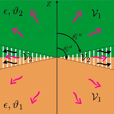
Figure 1 Diagram showing the regions V1 and V2 determined through the discarding angles θ0UH and θ0LH. The region V1, where only the spherical waves (undulated pink arrows) are taken into account is defined by θ0,θ0UHθ0LH,π. The region V2 (white hatched region), defined by θθ0UH,θ0LH, contains the intermediate region (s<s0=1) where both cylindrical waves (undulated black waves) and spherical waves have to be taken into account. Nevertheless, going further into the radiation zone for each observation point in the intermediate region one can make s>s0=1, thus making the cylindrical waves unobservable. 

To fix ideas let us consider now the UH and examine what happens when we fix the angle and explore the consequences changing the observation distance to a larger value r>>r0,i.e., we go farther into the radiation zone. Suppose that in the region V1 we consider the angle θ1<θ0UH, where we have s1=k~0r0(1-sinθ1)>1 according to our choices. Then, keeping θ1 fixed and going to a larger distance r>>r0 would only increase the value of s>=k~0r>(1-sinθ1) such that s>>s1>s0=1. That is to say, all observation points in V1 with r>r0 will have s>s0=1 and the cylidrical waves will not be relevant there.

On the other hand, the region V2 shows a mixed behavior. Again, let us consider an angle θ2>θ0UH where we have s2=k~0r0(1-sinθ2)<1 by construction. Nevertheless, an increase in the observation distance to r> can revert the situation yielding a value s>>1. To this end it is enough to take r>>r0/s2. That is to say, the region V2 contains the intermediate region where the cylindrical waves are relevant, but going further into the radiation zone these waves can be safely neglected. A similar situation occurs in the LH, which we do not discuss in detail here.

From the function erfc-iik~0r(1-sinθ) appearing in the Eqs. (22) and (23) we identify the analogous of the Sommerfeld numerical distance S in the standard dipole radiation, which is determined by rewriting the complementary error function as erfc (-iS)[13]. Thus we have

S=ik~0r(1-sinθ)=is2, (31)

which varies with the angle θ for a fixed observation distance r. This quantity is closely related to the discarding angle θ0 according to

|S|=1-sinθ1-sinθ0. (32)

Going back to the calculation of the electromagnetic field in the far-field approximation, we now write the corresponding expressions for the electromagnetic potentials obtained from plugging the results (22-24) into the (16-18). In the case of the region V1 we have

A0(x;ω)=-pn2ik~0cosθeik~0(r-z0cosθ)r-1n2θ~2p4n2+θ~2k~0sin2θ|cosθ|eik~0(r+z0|cosθ|)ir  , (33)

Aa(x;ω)=p4n2+θ~2-2θ~ik~0εabxbr+θ~2iω|cosθ|xareik~0(r+z0|cosθ|)r  , (34)

A3(x;ω)=-iωpeik~0(r-z0cosθ)r, (35)

where we dropped terms of higher order. On the other hand, in the intermediate region V2, (s > 1) the contribution of the cylindrical waves near the interface is apparent. The electromagnetic potential now is

A0(x;ω)=pn2ik~0ξeik~0(rz0ξ)r-1n2θ~2p4n2+θ~2k~0eik~0ririk~0z0-ξ8-1n2θ~2p4n2+θ~2k~022πik~0reik~0rπ2i+πik~0r2ξ  , (36)

Aa(x;ω)=p4n2+θ~2-2iθ~k~0εabxbρeik~0(r+z0ξ)r+θ~2iωxaρeik~0rrik~0z0-ξ8-θ~2ωk~0xaρ2πik~0reik~0rπ2i+πik~0r2ξ  , (37)

A3(x;ω)=-iωpeik~0(rz0ξ)r, (38)

where we again dropped terms of higher order. The minus (plus) sign in the first term of the right-hand side in Eq. (36) corresponds to the UH (LH), respectively. We have also performed a first order power expansion around π/2 in the complementary error function arising from Eqs. (22) and (23) in terms of the variable ξ<1 given by

ξUHπ/2-θUH,ξLH=θLH+π/2, (39)

for the UH and LH, respectively. Let us observe that for both hemispheres we have ξ>0 and also that (1-sinθ)=ξ2/2. In analogous way it is convenient to introduce the corresponding variable ξ0 related to the discarding angle θ0 just by replacing ξξ0 and θθ0 in Eq. (39). Using also Eq. (29) we obtain ξ0=2/(nωr0). In this way |S|=ξ2/ξ02<1 for both hemispheres. The expansion in powers of ξ is only valid in the intermediate zone where we have ξξ0.

3.2 The electric field

Since Faraday law yields B=ϵ n^×E in the far-field approximation we need to calculate only the electric field E(x;ω) to get a complete description of the radiation regime, where n^B=0 is satisfied. The components of the electric field are calculated through

E(x;ω)=-ik~0n^A0(x;ω)+iωA(x;ω)  . (40)

3.2.1 The region V1

Substituting in Eq. (40) the previous expressions for Aμ(x;ω) in the region V1 we obtain the following electric field:

Ea(x;ω)=-f(θ,z0,ω)zxar2+2θ~n4n2+θ~2eik~0z0|cosθ|εabxbrω2peik~0rr,E3(x;ω)=sin2θ f(θ,z0,ω)ω2peik~0rr, (41)

with

f(θ,z0,ω)=e-ik~0z0cosθ+sgncosθθ~24n2+θ~2eik~0z0|cosθ|. (42)

Here sgn denotes the sign function with the additional condition sgn(0) = 0. It is possible to verify that n^E=0 as required for the electric field in the far-zone regime. The main feature in the components of the electric field (41) is the presence of two different phases in the exponential related to the source variables x'=z0 z^, which are specified by cosθ and |cosθ| as shown in Eq. (42). The first exponential contributes with the term expik~0r-z0cosθ having the characteristic phase of dipole radiation in standard electrodynamics [35,37]. On the other hand, the contributions arising from the new terms involving the MEP, which are proportional to θ~ and θ~2, yield the exponential expik~0r+z0|cosθ|. As we will show in the next subsection, the modifications in the power spectrum of the dipolar radiation in our setting arise precisely due to the contribution z0|cosθ| in the phase of the electric field. The dependence on the sign of cosθ enforces two cases, which we denote as Case (—) and Case (+). The former case occurs when |cosθ|=-cosθ, i.e. when θ(θ0LH,π[ is in the LH. In this situation the three components of the electric field will have the same phase and we do not expect significant changes with respect to the usual angular dependence of the dipolar radiation because the phase of the electric field is that of standard electrodynamics. By contrast, the Case (+) takes place when cosθ=cosθ, which is realized for θ[0,θ0UH) in the UH. In this case the electric field presents two different phases which will interfere yielding new effects different from those in the usual dipolar radiation.

Finally, we analyze the function f(θ,z0,ω) given by Eq. (42), which codifies the different phases of the electric field (41). For the Case (+), f takes the following form

f+(θ,z0,ω)=f(θ,z0,ω)|UH=e-ik~0z0cosθ+θ~24n2+θ~2eik~0z0cosθ. (43)

On the other hand, for the Case (—), the function f is

f-(θ,z0,ω)=f(θ,z0,ω)|LH=4n24n2+θ~2e-ik~0z0cosθ. (44)

In the following we show that the factors θ~2/(4n2+θ~2),  4n2/(4n2+θ~2) and 2θ~/(4n2+θ~2) correspond to some reflection and transmission coefficients at the interface. Let us start with the radiation fields in the UH by considering the general expression for the reflected electric field discussed in the Appendix B of Ref. [48], where the authors calculate the GF of a planar interface separating two semi-infinite TIs. The reflective part of such GF is written as

Gij(x,x';ω)=d2k(2π)2eikRRij(k,kz,z,z')  , (45)

which connects the electric field components Ei directly with the current density jk through the equation

Ei(x;ω)=-4πiωd3x'Gik(x,x';ω)jk(x';ω)  . (46)

In our case only j3=-iωpδ(x')δ(y')δ(z'-z0) is different from zero so that the only contributions to Rij come from Ri3, which can be read from Eqs. (B8), (B10) and (B12) of Ref. [48] for an incident TM polarized plane wave, and which we rewrite here

R13(k,kz,z,z0)=ieikz(z+z0)2kz-kxkzk2RTM,TM+kykRTE,TM  , (47)

R23(k,kz,z,z0)=ieikz(z+z0)2kz-kykzk2RTM,TM-kxkRTE,TM  , (48)

R33(k,kz,z,z0)=ieikz(z+z0)2kzk2k2RTM,TM. (49)

Incidentally, the above equations show that the TM and TE polarizations are mixed as a consequence of the MEE. The explicit expressions for the reflection coefficients are given in Eqs. (44)-(46) of Ref. [48]. The notation in Ref. [48]{k,kp,kz} is equivalent to ours k~0,k,k~02-k2, respectively. In this way, the components of the electric field are

E1(x;ω)=-4πiω2p    d2k(2π)2eikzz02kz-kxkzk2RTM,TM+kykRTE,TMeikReikzz, (50)

E2(x;ω)=-4πiω2p    d2k(2π)2eikzz02kz-kykzk2RTM,TM-kxkRTE,TMeikReikzz, (51)

E3(x;ω)=-4πiω2p    d2k(2π)2eikzz02kzk2k2RTM,TMeikReikzz. (52)

To compute the far-field approximation of the electric field written above, which is necessary to compare with our expressions (41) and (42), we make use of the angular spectrum representation method which we briefly review [49]. For fields satisfying the Helmholtz equation (2+κ2)E=0, with κ2=ϵω2, which can be written as

Ei(x,y,z)=d2kE^i(kx,ky,z)eikx, (53)

one can show that

E^i(kx,ky,z)=E^i(kx,ky,z=0)e±ikzz,kz=κ2-k2,Im(kz)0, (54)

choosing the +, — signs according to z > 0 or z < 0, respectively. Substituting Eq. (54) into Eq.(53) yields the so-called angular spectrum representation of the electric field. One of the notable consequences of this approach is that the far-field approximation of the electric field is given in terms of the function E^kx,ky,z=0. According to Ref.[49] we have

Ek~0rxr,yr,zr=-2πik~0szE^(kx=k~0sx,  ky=k~0sy,  z=0)eik~0rr,

sx=sinθcosφ,sy=sinθsinφ,sz=cosθ,kz=k~0sz=k~0cosθ. (55)

Our next step is to identify the respective functions E^i(kx,ky,z=0) in each of the components (50)-(52), so that we can apply the relation (55). Making the required substitutions we find that

E^i(kx,ky,z=0)=-iω2p2πkzeikzz0[    ]i, (56)

where each square bracket [   ]i denotes the corresponding one in Eqs. (50)-(52). Substituting in (55) yields

Ek~0r1=xzr2RTM,TM-yrRTE,TMpω2eik~0rreik~0cosθz0, (57)

Ek~0r2=yzr2RTM,TM+xrRTE,TMpω2eik~0rreik~0cosθz0, (58)

Ek~0r3=-|x|2r2RTM,TMpω2eik~0rreik~0cosθz0,        |x|2r2=sin2θ.         (59)

Comparing the above results with our expressions (41) and (42) for f+ yields the identifications

RTM,TM=θ~24n2+θ~2,RTE,TM=-2θ~n4n2+θ~2. (60)

Carrying the analogous calculation for the LH with f-, we read the transmission coefficients

TTM,TM=4n24n2+θ~2,TTE,TM=RTE,TM. (61)

We immediately verify that RTM,TM+TTM,TM=1 as expected. Let us observe that the expressions for the transmission and reflection coefficients obtained from our calculation can be verified from the general expressions (43)-(46) in Ref. [48], after the following restrictions are made: ϵ1=ϵ2=ϵ=n2, μ1=μ2=1, kz1=kz2=kz and Δ=θ~.

3.2.2 The intermdiate zone in the region V2

Let us recall that for any observation point in V2 with s<s0=1 we can go farther into the radiation zone and find s>>1, thus eliminating the cylindrical waves. In this subsection we deal only with the region having s<s0=1. This region corresponds to what is normally called the intermediate region in the literature [13] and is characterized by the condition that the Sommerfeld numerical distance S=is2 satisfies |S|<1, in spite of k~0r being large. Clearly this is possible because we are in the limit θπ/2, (ξ0),i.e. very close to the interface.

A precise characterization of the intermediate zone in the UH is provided as follows: According to our criterion (30), which is written there for an arbitrary s0, we choose s0=1 as the specific value for this parameter. Then, for r0 in the radiation zone (k~0r01) the discarding angle θ0 is determined such that s0=k~0r0(1-sinθ0UH). For angles θ0UH<β<π/2 we have 0<sβ=k~0r0(1-sinβ)<s0. Within this angular range we still can move further into the radiation zone to rβ, within the interval r0<rβ<r0 (s0/sβ), where cylindrical waves are still present and which define the intermediate zone.

So, in this region the electric field is

Ea(x;ω)=ξxaρ eik~0z0ξ+2θ~ n4n2+θ~2εabxbρeik~0z0ξp ω2 eik~0rr  ,

E3(x;ω)=eik~0z0ξr±θ~24n2+θ~2k~0ξiz0r+π22πik~0r p ω2eik~0r, (62)

where we have dropped terms Oξ2. The variable ξ was previously defined in Eq. (39) for each hemisphere. Also we verified that n^E=0 using the approximations sinθ1 and cosθξ, which are adequate for the region V2. From Eq. (62) we observe the presence of cylindrical waves, codified in the term proportional to eik~0r/r[6], where we notice that rρ close to the interface. They are also present in the standard case of dipolar radiation when two different electromagnetic media are separated by a planar interface. Nevertheless, in our case they only contribute when at least one of the media is magnetoeletric, i.e. when θ~0 defines the interface. This is because we have chosen two non-magnetic media with the the same permittivity ϵ, which means that setting θ~=0 yields an infinite media with no interface at all. The subject of cylindrical waves in dipole radiation has been exhaustively discussed in the literature been a highly controversial topic. An authoritative discussion of this case, including an historical perspective, can be found in Subsec.4.10 of Ref. [13].

We finalize this section by presenting plots for the real part of the electric fields (41) and (62) in their corresponding regions V1 and V2. These plots will provide a quantitative behavior of the electromagnetic field and reinforce the space splitting exposed in Fig. 1. Figures 2a) and 2b) show the x and y components, respectively, and Figs. 2c) and 2d) are devoted to the z component. All the figures represent the real part of the electric field (equivalent to the time dependent field at t = 0) in the x - z plane. Here the interface is constituted by a normal insulator with ϵ=4 and ϑ2=0 in the UH and a medium with ϵ=4 and ϑ1=5 in the LH to make evident the new effects. The dipole has a strength p=2.71×10³eV-1, a frequency ω=1.5eV and is located at z0=25eV-1 (an explanation of this parameters choice will be given in the Subsec. 4.1 immediately below). The field patterns for the x and z components in Figs. 2a), 2c) and 2d) show different behaviors at both sides of the interface. Indeed, in the upper semi-space the effect of the interference between the two phases of the electric field associated to the Case (+) is quite appreciable. Regarding the lower semi-infinite space, the features of the Case (—) are visible, because one observes clearly the absence of an interference pattern and the same behavior of an electric dipole field. Remarkably the y component in Fig. 2b), which is different from zero in comparison with the usual electric dipole radiation, results proportional to θ~ and does not exhibit an interference pattern due the vanishing of the first term of Eq. (41) at the x - z plane.

Figure 2 The electric field pattern (real part) in the x - z plane for a vertically oriented point dipole with single frequency ω=1.5 eV, strength p=2.71×10³  eV-1 and located at z0=25eV-1 close to a magnetoelectric interface, for the region V1 where only the spherical waves are significant. Here the UH is a normal insulator with ϵ=4 and ϑ2=0 and the LH is a medium with ϵ=4 and ϑ1=5. The plots a) and b) are the x and y components respectively. The plots c) and d) are the z components in the UH with discarding angle θ0UH1.5391888.19 and in the LH with discarding angle θ0LH1.6024191.81 respectively. 

Recalling from Eq. (62) that only the z component of the electric field contributes to the cylindrical waves, we need to employ the discarding angles given by Eqs. (29) to split the space into the regions V1 and V2 of Fig. 1. Figure 2c) illustrates this splitting for the z component in the UH for angles in the range θ[0,θ0UH) with θ0UH1.5391888.19 and Fig. 2d) shows the same but in the LH for angles in the range (θ0LH,π] with θ0LH1.6024191.81. Conversely, Figs. 3a) and 3b) show the behavior of the z component in the UH for angles in the range θ[θ0UH,π/2) and in the LH for angles in the range θ[π/2,θ0LH], respectively. Here the appearance of the axially symmetric cylindrical waves is clear, although our plots show that they are confined to a finite distance range and decay rapidly for large distances parallel to the interface. The discarding angles are not to scale for the purpose of making evident the appearance of cylindrical waves. Our approximation yields zero for the x and y components of the electric field in the region V2.

Figure 3 The electric field pattern (real part) in the x - z plane for a vertically oriented point dipole with single frequency ω=1.5eV, strength p=2.71×10³  eV-1 and located at z0=25eV-1 close to a magnetoelectric interface, for the region V2 where the spherical waves and the cylindrical waves are significant. Here the UH is a normal insulator with ϵ=4 and ϑ2=0 and the LH is a medium with ϵ=4 and ϑ1=5. The plots a) and b) are the z components in the UH and in the LH respectively. The discarding angles are θ0UH=88.19 and θ0LH=91.81, which are not to scale for the purpose of making evident the presence of cylindrical waves. 

4 Angular distribution, total radiated power and energy transport

4.1 The parameters

With the purpose of illustrating our results with some numerical estimations we need to fix the parameters defining our setup. Our choice is motivated by the fact that current magnetoelectric media are of great interest in atomic physics and optics, therefore we think as a dipolar source an atom with a given dipolar moment p, whose emission spectrum goes from the near infrared to the near ultraviolet. Furthermore, the magnetoelectric coupling is usually very small (of the order of the fine structure constant for TIs), so that appreciable effects will appear near the interface. In this way we have chosen the distance between the dipole and the observer to be lesser than 1 mm. For all cases in the following numerical estimations, with the exception of Fig. 6, we take the frequency ω=1.5eV (362.7 THz or λ=826.6 nm) in the near infrared, the observer distance r=667eV-1 (0.131 mm), and the dipole location at z0 = 25eV-1 (4.94 μm). The far-field condition is well satisfied with nωr1000 n. The remaining free parameters are θ~ and n, which characterize the medium. This setup provides a microscopic antenna in front of a magnetoelectric medium. The additional boundary conditions at the interface drastically modify the dominant dipolar radiation. These changes can be directly observed by measuring the angular distribution of the radiation, which looks feasible having in mind similar techniques developed in Refs. [50,51]. Another possibility is to observe the modified radiative lifetime of the atom, which must change due to the dominance of the modified dipolar radiation [52]. These effects have been already demonstrated in experiments [53,54].

4.2 Angular distribution for the radiation in the region V1

In this subsection we obtain the angular distribution of the radiated power associated to the electric field given by Eqs. (41) for the region V1. Recalling that the electromagnetic fields satisfy n^E=0 and B=ϵ n^×E we obtain the standard Poynting vector in a material media with μ = 1,

S=14πE×H=ϵ4πE2n^, (63)

where n^ coincides with the direction of the phase velocity of the outgoing wave. According to Refs. [35,37], the time-averaged power radiated per unit solid angle solid by a localized source is

dPdΩ=r22ReE(x;ω)×H*(x;ω)4π=nr28πE(x;ω)E*(x;ω). (64)

The result for our dipole p is

dPdΩ=nω4p28πsin2θ{1+Υ sgn2cosθ+2Υ sgn×cosθcosk~0z0|cosθ|+cosθ},     (65)

where Υ=θ~2/(4n2+θ~2). Some comments regarding this angular distribution are now in order. The expression (65) is an even function of the MEP θ~ as well as of the angle θ. Furthermore, the last term in Eq. (65) arises from the interference between the two different phases exhibited by the electric field in Eq. (41) and could or could not contribute depending on the sign of cosθ.

At this stage it is important to emphasize that our result in Eq. (65) shows that Υ sets the scale in the magnitude of the power radiated in the region V1. This parameter has the relevant property of being bounded within the interval 0<Υ<1, independently of the values which θ~ and n might take. This will severely constrain the response of the ϑ-medium with respect to the output produced by an electric dipole in an infinite media with refraction index n. We refer to the latter reference setup as the standard electrodynamics (SED) case, which is obtained setting θ~=0 in Eq. (65) yielding the well known dipolar angular distribution [35].

Now, we analyze the angular distribution of the radiated power (65) for the Case (—) discussed in Sec. 3.2.1, when the electric field has a single phase. Making this choice in Eq. (65), we obtain

dP(-)dΩ=nω4p28πsin2θ(1-Υ). (66)

Notice that the factor (1-Υ)=4n2/(4n2+θ~2) is always positive which confirms a basic property of the radiated power. We observe that the angular dependence of the radiated power remains unchanged with respect to the SED case, confirming what we found at the level of the electric field in Figs. 2a) and 2d). Nevertheless, the magnitude of the radiation turns out to be smaller for a fixed angle, which provides a fundamental difference with respect to this reference setup. Surprisingly, in the highly hypothetical situation where Υ1, the radiation in the LH would be completely canceled i.e. the setup would behave as a perfect mirror.

On the other hand, for the Case (+), when the electric field includes two different phases, we obtain the angular distribution

dP(+)dΩ=nω4p28πsin2θ×1+Υ+2Υcos2k~0z0cosθ, (67)

which present additional contributions to the angular distribution with respect to those in SED. They arise from the last term in Eq. (67). Furthermore, as opposed to the previous case, the angular distribution now depends explicitly on the dipole position z0. Let us observe that the minimum value -1 of cos(2k~0z0cosθ) produces the factor (1-Υ) in the square bracket, which was discussed above.

The behavior of the angular distribution (67) is shown in Fig. 4. In each case, the electric dipole is located at z0 > 0 and the interface corresponds to the line (3π/2-π/2) defining z = 0. The Fig. 4a) is plotted for the ϑ-medium TbPO4 with n = 1.87 [55] and θ~=0.22[56]. After comparing with the SED case we appreciate only weak signals of interference. The Fig. 4b) corresponds to an hypothetical material with θ~=0.5 and n = 2. Finally, in Fig. 4c we see a clear enhancement in the interference pattern for our electric dipole radiating in front of an another hypothetical material with θ~=1 and n = 2. An increasing value of the parameter θ~ in Fig. 4 makes evident the interference effects, which are expected to be more pronounced in the vicinity of θ=π/2 where the last term in Eq. (67) oscillates maximally. This interference effect agrees with our results plotted in Figs. 2a) and 2c).

Figure 4 Angular distribution of the radiated power dP(+)/dΩ. a) Polar plot with θ~=0.22, n=1.87, b) Polar plot with θ~=0.5, n=2. c) Polar plot with θ~=1, n=2. The scale is normalized by multiplying dP(+)/dΩ by 4π/ω4p2. The remaining parameters ω=1.5 eV, r=667 eV-1, z0=25 eV-1 are common to this and all subsequent figures. 

Even though the method of images does not generalize to the time dependent case, a qualitative interpretation for the radiation patterns described above can be given by extending to the quasi-static approximation the characterization of a point charge located in front of a magnetoelectric medium in terms of electric and magnetic images presented in detail in Ref. [57]. In this way, the full description of the MEE of a dipole located in front of a planar medium includes electric and magnetic image dipoles. Let us first deal with the Case (—), which corresponds to the situation when the electric dipole and the observer are in different semi-spaces, i.e. the dipole is located at r0=(0,0,z0) with z0 > 0 and the observer’s angle θ is in the LH. The MEE is mimicked by introducing an image dipole p’ and an image magnetic dipole m both located at r0, i.e. in the same semi-space and in the same position of the electric dipole p. So, the observer will measure the same phase of the radiation from p, p’ and m, which is given by choosing |cosθ|=-cosθ in the phase of the electric field (41). This sign choice affects the angular distribution (65) by canceling the interference term, as Eq. (66) shows. Therefore, the angular dependence of the radiation that the observer detects will not present a substantial difference from that of SED, as Figs. 2a) and 2d) can also confirm. Let us recall that we have chosen the two non-magnetic media having the same permittivity, which eliminates the optical refraction and reflection phenomena when passing from one magnetoelectric medium to the other. On the other hand, the Case (+) can be understood in a similar way. Here both objects, electric dipole and observer, are in the same semi-space and the observer’s angle θ is in the UH. Again we emulate the MEE by inserting an image dipole p’ and the same image magnetic dipole m [57], both localized at -r0. In this way, the observer will detect radiation with two different phases: one from the source electric dipole and another from the image objects p’ and m, which corresponds to the choice |cosθ|=+cosθ in the phase of the electric field (41). The plus sign selection impacts significantly the angular distribution (65) because the interference term is now non-zero and contributes to observable quantities as shown in Eq. (67) together with Figs. 2a), 2c) and 2d). This interference arises between the radiation coming from bottom to top, generated by the image objects, and the direct signal from the dipole source and generates a different angular dependence in the UH when compared with the electric dipolar radiation of SED. Both cases are schematically illustrated in Figs. 5a) and 5b), respectively.

Figure 5 a) Illustration of the Case (—), where the radiation (black thick arrows) has a single phase, which is the one of standard ED, when the observer O1 is in a different semi-space with respect to the dipole p at z0. b) In the Case (+) (observer O2 in the same semi-space of the dipole) the radiation seen by O2 includes two different phases: the one arising from p at z0 and the other that comes from the images p’ and m at —, z0. Recall that we have two non-magnetic media with ϵ1=ϵ2, which yield no refraction at the interface. 

4.3 Power radiated in the region V1

In order to compare the magnitude of the radiation in the ϑ-medium with respect to the SED case it is convenient to introduce what we call the enhancement factor R(±) defined as R(±)=2P(±)/P0, where P0=nω4p2/3 is the total power radiated by an electric dipole in the SED case [35].

Next we calculate the power radiated for the angular distributions (66) and (67) in the region V1. Let us begin with the angular distribution of the Case (—) given by Eq. (66). Integrating over the solid angle Ω for θ(θ0LH,π and ϕ0,2π, we find the radiated power

P(-)=P02(1-Υ)1+98cosθ0LH-18cos3θ0LH. (68)

A good estimation of the enhancement factor is obtained writing θ0=π/2+ξ0 and recalling that ξ0<1. We obtain

R(-)=(1-Υ)1+3ξ02. (69)

which can be larger (smaller) than one according to Υ<3 ξ0/2(Υ>3 ξ0/2 ), respectively. In the hypothetical limit θ~2n we have Υ=1 and there is no radiated power in the LH, which tells us that the setup behaves like a perfect mirror as discussed in the previous section.

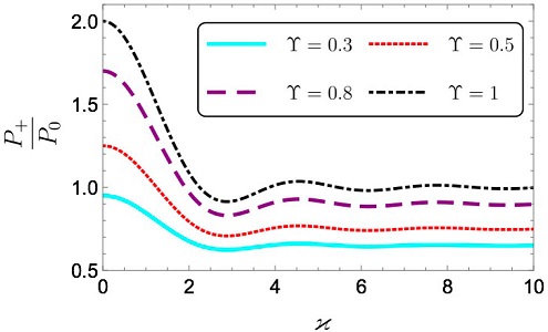
Now, we repeat the calculation for the angular distribution of the Case (+) given by Eq. (67), which is more interesting. After integrating over the solid angle Ω for θ0,θ0UH, the power radiated P(+) is

P(+)=P02(1+Υ)1-98cosθ0UH+18cos3θ0UH+P023Υsin(2ϰ)4ϰ3-cos(2ϰ)2ϰ2+cosθ0UHcos(2ϰcosθ0UH)2ϰ2-1+ϰ2-ϰ2cos(2θ0UH)sin(2ϰcosθ0UH)4ϰ3,ϰk~0z0. (70)

The main difference with respect to the power radiated in the LH is that now P(+) depends on the position of the dipole through the variable ϰ. The power radiated P(+) is positive definite and due to the term in braces we expect to find new effects in comparison with the previous Case (—). Moreover, from Eq. (70) and retaining n and ω fixed we find the following interesting limits for z0

P(+)z0=P02×(1+Υ)1-98cosθ0UH+18cos3θ0UH, (71)

P(+)z00=P02(1+3 Υ)×1-98cosθ0UH+18cos3θ0UH+P02  25Υ  ϰ2(5cos3θ0UH-3cos5θ0UH-2),ϰ1. (72)

The Eq. (72) tells us that there are no divergences in Eq. (70) when the electric dipole is very close to the interface. Since for all practical purpose θ0UH is very close to π/2, we obtain a very good approximation of P(+) in the intricate Eq. (70) by setting θ0UH=π/2, which yields the simplified expression

P(+)=P021+Υ1+3sin2ϰ4ϰ3-3cos2ϰ2ϰ2. (73)

As we can calculate from Eq. (73), the enhancement factor R(+)=2P(+)/P0 has the following properties. The maximum occurs when the dipole is at the interface (ϰ=0) and yields R(+)max=1+3Υ. Also we found an absolute minimum located at ϰ2.88 where R(+)min=1+0.83 Υ. The limit for very large ϰ is R(+)=(1+Υ). In the Fig. 6 we plot the ratio P(+)/P0 in the approximation of Eq. (73), as a function of ϰ for different choices of the parameter Υ, which provides a qualitative confirmation of the behavior of R(+) discussed above.

Figure 6 Plot of P(+)/P0 as a function of ϰ for different choices of Υ. The enhancement factor is R+=2P+P0.  

4.4 Energy transport in the intermediate region of V2

In this subsection we discuss the energy flux in the region V2 when s>s0=1 and the spherical and cylindrical waves coexist as shown in Eq. (62). This region was fully characterized previously in the paragraph before Eq. (62).

As pointed out in Ref. [47], the separation of the electric field (62) in these two components is not significant since they do not constitute independent solutions of Maxwell equations. Recalling Eq. (63) for the time-averaged Poynting vector S we obtain

SV2UH=n^np2ω48π{1r21+4θ~2n2(4n2+θ~2)2+ω1/2r3/2θ~24n2+θ~2n π ξ}+O(ξ2), (74)

SV2LH=n^np2ω48π{1r21+4θ~2n2(4n2+θ~2)2-ω1/2r3/2θ~24n2+θ~2n π ξ}+O(ξ2), (75)

to first order in ξ. In the above linear expansion we require

nωz0ξ    1. (76)

We observe that these fluxes are independent of the position of the dipole. In Eqs. (74) and (75) we encounter two different terms: one modulated by r-2 which contains the energy flux coming from the spherical wave contribution, and another one proportional to r-3/2 that encodes the interference between the spherical and cylindrical waves. The contribution of the cylindrical wave itself is of order ξ2 which we have consistently neglected in our approximation.

Two remarks are now in order: (i) For a fixed set of parameters, Eqs. (74) and (75) yields SV2UH-SV2LH>0. (ii) The full expression for the energy flux must be positive definite, but we are dealing only with a linear approximation in Eq. (75). This forces us to establish an additional bound for the validity of our results. The dangerous contribution is in SV2LH, where the relative minus sign might produce a negative value. Recalling that ξ0=2/(nωr0), defined after Eq. (39), we rewrite the resulting condition from Eq. (75) as

ξξ0<12π(4n2+θ~2)2+4n2θ~2θ~2(4n2+θ~2)r0r1/2<12π1+Υ-Υ2ΥQ(Υ),θ~0, (77)

since r>r0 in the intermediate zone. Recalling that 0<Υ<1, the function Q(Υ) is a decreasing function having its minimum value Q(Υ=1)=0.40. This means that for any value ξ/ξ0<0.40, the energy fluxes are always positive in the whole range of Υ since the inequality (77) is always satisfied.

On the contrary, when 0.40<ξ/ξ0ζ<1 we have to determine the maximum allowed value Υmax by solving QΥmax=ζ, so that the energy fluxes are positive only in the range 0<Υ<Υmax. Let us notice that the lowest values observed for θ~ are of the order of the fine structure constant α=1/137, which effectively replaces the theoretical lower limit Υ=0 by the more realistic one Υmin=1.3×10⁻⁵/n2.

Next we perform some numerical estimations of Eq. (75) shown in Table I. There we refer to the setup described in the beginning of Sec. 2, for the case where medium 1 is a regular insulator with n = 2(1.87, ), μ = 1 and ϑ = 0, while medium 2 corresponds to different magnetoelectric media with the same refraction index and permeability and whose value of θ~ is indicated in the third column. Since we are interested only in the magnetoelectric response of the real materials listed in Table I it is enough to say that TbPO4 is an antiferromagnet exhibiting a linear MEE, whose relevant properties have been extensively studied in Ref. [55,56]. On the other hand TlBiSe2 has been experimentally identified as a TI admitting MEPs given by θ~=(2n+1)π[58,59,60]. Its electronic properties are presented in [61]. The remaining entries correspond to hypothetical materials aiming to illustrate the effects of increasing the strength of the MEE. For this reason we take them with the same refraction index n = 2. We compare these fluxes with the magnitude of SSED written in the last column. We recall the dipole characteristics p=2.71×10³ eV-1  (10-21 Ccm), ω=1.5eV, z0=25eV-1 and the observer distance r=667 eV-1. In this case ξ0=3.2×10⁻². We present the magnitude of the Poynting vector SV2 for both hemispheres evaluated at ξ=10-3, which we choose as a representative value satisfying the condition (76) with nωz0ξ=7.5×10⁻², as well as ξ/ξ0=3.1×10-2, for n2. This latter number indicates that the condition (75) is fulfilled for all values of Υ in this case.

Table I The energy flux very close to the interface (ξ=10-3) between a normal insulator (n=2 (1.87),ϑ~=0, μ=1) and different magnetoelectrics with the same n and μ. The radiating dipole has p=2.71×10³  eV-1, ω=1.5 eV and z0=25eV-1. The observer distance is r=667 eV-1.  

ϑ-medium n θ~ Υ SUH  [eV4] SLH  [eV4] SSED  [eV4]
TlBiSe2 2 11α 4.0×10⁻⁴ 6.64 6.64 6.63
TbPO4 1.87 0.22 3.5×10⁻³ 6.21 6.21 6.18
Hyp. I 2 0.5 1.5×10⁻² 6.74 6.73 6.63
Hyp. II 2 1 5.9×10⁻² 7.03 6.97 6.63
Hyp. III 2 5 6.1×10⁻¹ 8.53 7.89 6.63

5 Summary and conclusions

We discuss the radiation produced by a point-like electric dipole oriented perpendicular to and at a distance z0 from the interface which separates two planar semi-infinite non-magnetic magnetoelectric media with the same permittivity, whose electromagnetic response obeys the modified Maxwell equations (4) and (5) of ϑ-electrodynamics. The choice ϵ1=ϵ2 is made to highlight and isolate the purely magnetoelectric effects on the radiation, which depend on the parameter θ~=α(ϑ2-ϑ1)/π. As a consequence of a careful calculation of the far-field approximation in the electric field we discover the additional generation of axially symmetric cylindrical (surface) waves close to the interface, as shown in Eqs. (62). The analysis of the cylindrical waves leads us to introduce two discarding angles θ0UH and θ0LH, defined in Eq. (29) and shown in Fig. 1, which allow to distinguish two separate regimes: i) the region V1, 0<θ<θ0UH,  θ0LH<θ<π, where only the spherical waves are relevant and ii) the region V2, (θ0UH<θ<θ0LH), where both the cylindrical and the spherical waves must be taken into account. The behavior of the electric field in region V1 and V2 is illustrated in Figs. 2 and 3, respectively.

Due to the presence of the ϑ-media we find modifications in the angular distribution of the radiation given by Eq. (65) and illustrated in Fig. 4. Noticeable interference effects are manifest in the upper hemisphere when the observer is in the same region of the dipole. On the contrary, no interference occurs when the observer and the dipole are not in the same region, in which case the angular distribution looks similar to that of a dipole in a homogeneous media, except for important changes in its magnitude. Such different interference effects say that the system distinguishes whether the electric dipole and the observer are in the same semi-space or not, corresponding to the Cases (+) and (—) respectively, discussed at the end of Subsec. 4.2.

Starting from the far-field approximation of the electric field we have correctly identified the Fresnel coefficients at the interface by making use of the angular spectrum representation [49] together with the results of Ref. [48] dealing with wave propagation in layered topological insulators.

The modifications of the angular distribution in the region V1 produce new expressions for the total radiated power P(±), which were calculated in Eqs. (68) and (70). The result P- for the lower hemisphere is independent of the dipole’s location z0 and shows a behavior similar to the standard electrodynamics configuration, but modulated by two amplitudes. The amplitude depending on the discarding angle θ0LH is very close to one, because for all practical purposes θ0LH=π/2. The second amplitude depends on Υ and induces an unexpected behavior yielding an enhancement factor R(-) that can be less than one in some cases. Further, in the limiting case when Υ1 the radiation in the lower hemisphere would be completely canceled, such that the setup behaves as a perfect mirror. The result for P(+) is more intricate since the dependence upon z0 now survives in the angular distribution of Eq. (65). Again, the discarding angle is very close to π/2 and we take this approximation to obtain some general features of the enhancement factor. We find the maximum value R(+)=1+3Υ, when the dipole is located at the interface (z0 = 0). In the limit ϰ=nωz0 very large we have R(+)1+Υ. Also we find an absolute minimum at ϰ2.88 where R(+)=1+0.83 Υ. Thus, in this case we have an enhancement factor larger than one, which nevertheless is limited to the maximum value of R(+)max=4, independently of our choice of the parameters θ~ and n of the medium. In Fig. 6 we plot the ratio P(+)/P0 as a function of ϰ, for different choices of Υ, where P0 stands for the total power radiated by the dipole in standard electrodynamics.

Regarding the region V2, we have carefully characterized along the text the conditions under which the cylindrical waves arise. The cylindrical waves are present in the whole interval 0<ξ<ξ0, |s|<1 so that |S|=ξ2/ξ02<1 for both hemispheres in this region. Our linear approximation in ξ, carried out in Eqs. (74) and (75), is only valid when ξξ0, and the effect of the ϑ-medium is again codified in the parameter Υ. As expected, the effects of the magnetoelectric become more evident for large θ~. The fluxes in both hemispheres are larger than in the standard electrodynamics configuration and the excess of radiation in the upper hemisphere with respect to the lower hemisphere is evident in Table I.

In order to stress their similarities and differences we give some comparison between the dipolar radiation studied in this work which includes a magnetoelectric medium, and that produced in the presence of two standard insulators with a planar interface and different permittivities ϵ(x)=Θ(z)ϵ2+Θ(-z)ϵ1 with ϵ1ϵ2 and ϑ1=ϑ2=0. In the latter case the radiation of a vertically oriented dipole picks up only the TM polarization as shown in Refs. [44,49]. In our case we have identified these contributions to the electric field through the corresponding transmission TTM,TM and reflection RTM,TM coefficients in Eqs. (60) and (61). However, due to the magnetoelectric effect, the electric field gets an additional input arising from the mixing of TM and TE modes described by the reflection coefficient RTE,TM in Eq. (60). While in purely dielectric configuration these coefficients have an angular dependence, in our case they turn out to be constants depending only on the parameters of the media. This is a consequence of our choice ϵ1=ϵ2, which forbids the existence of reflection and refraction at the interface. On the other hand, both configurations share the generation of axially symmetric cylindrical waves at the interface of the two media, as shown in Subsec. 3.2.2 and particularly in Fig. 3. Again, in our case the physical origin of such cylindrical waves relies on the change in the magnetoelectric polarizability across the two media and not because of a difference in the permittivity constant as it happens in the purely dielectric configuration.

Let us emphasize once again that our methods can be applied to study the radiation in all materials whose macroscopic electromagnetic response is described by ϑ-electrodynamics. This includes any magnetoelectric medium, which can be found among a wide range of ferromagnetic, ferroelectric, multiferroic materials and topological insulators, for example. Our results contribute to the list of uncovered consequences of the magnetolelectric effect, which still remains far from experimental confirmation. Generally speaking, the parameter α~αϑ/π (in Gaussian units) which sets the scale for the magnetoelectric effect via the constitutive relations (3) is very small. Then is is clear that to enhance such effects, materials with much higher magnetoelectric polarizabilities are required. Besides those values previously mentioned in the text, some typical values are: 2.8 × 10⁻² for MgO/Fe [62] and 7.2 for Gd2O3/Co [63]. Nonetheless, the search for a giant magnetoelectric polarizability continues recently in composite materials reaching values as high as 9.0 ×10² for BaTiO3/Co60Fe40, for example [64]. Among the numerous technological applications envisaged as a consequence of the magnetoelectric effects we mention just a few: electric field control of magnetism, low-energy-consumption non-volatile magnetoelectronic memory devices, high sensitivity magnetometers, microwave frequency transducers and spintronics for future photonic devices [65,66,67]. Nevertheless, all these possibilities crucially depend on finding materials with higher and higher magnetoelectric polarizabilities.

Acknowledgments

OJF has been supported by the postdoctoral fellowship CONACYT-770691 and the doctoral fellowship CONACYT-271523. OJF and LFU acknowledge support from the CONACYT project #237503 as well as the project DGAPA-UNAM-IN103319. LFU acknowledges also support from the project CONACyT (México) # CF-428214. LFU and OJF thank Professor Rubén Barrera, Prof. Hugo Morales-Técotl, Dr. Alberto Martín-Ruiz and Dr. Omar Rodríguez-Tzompantzi for useful discussions and suggestions. OJF thanks Dr. J. A. Crosse for his useful help to plot the electric fields.

References

1. K.A. Michalski and J. R. Mosig, The Sommerfeld half-space problem revisited: from radio frequencies and Zenneck waves to visible light and Fano modes, Journal of Electromagnetic Waves and Applications, 30:1 (2016) 1. https://doi.org/10.1080/09205071.2015.1093964. [ Links ]

2. T.I. Jeon and D. Grischkowsky, THz Zenneck surface wave (THz surface plasmon) propagation on a metal sheet, Appl. Phys. Lett. 88 (2006) 061113. https://doi.org/10.1063/1.2171488. [ Links ]

3. L. Novotny, Allowed and forbidden light in near-field optics. I. A single dipolar light source, J. Opt. Soc. Am. A 14 (1997) 91. https://doi.org/10.1364/JOSAA.14.000091. [ Links ]

4. S.A. Maier and H.A. Atwater, Plasmonics: localization and guiding of electromagnetic energy in metal/dielectric structures, Journal of Applied Physics 98 (2005) 011101. https://doi.org/10.1063/1.1951057. [ Links ]

5. R. Gordon, Surface plasmon nanophotonics: A tutorial, IEEE Nanotechnology Magazine 2 (2008) 12. https://doi.org/10.1109/MNANO.2008.931481. [ Links ]

6. A. Sommerfeld, Über die Ausbreitung der Wellen in der drahtlosen Telegraphie, Ann. Physik 28 (1909) 665. https://doi.org/10.1002/andp.19093330402. [ Links ]

7. H. v. Hörschelmann, Über die Wirkungsweise des geknickten Marconischen Senders in der drahtlosen Telegraphie, Jb. drahtl. Telegr. u. Teleph. 5 (1911) 14 and 188. [ Links ]

8. A. Sommerfeld, Über die Ausbreitung der Wellen in der drahtlosen Telegraphie, Ann. Physik 81 (1926) 1135. https://doi.org/10.1002/andp.19263862516. [ Links ]

9. H. Weyl, Ausbreitung elektromagnetischer Wellen über einem ebenen Leiter, Ann. Physik 60 (1919) 481. https://doi.org/10.1002/andp.19193652104. [ Links ]

10. M.J.O. Strutt, Strahlung von Antennen unter dem Einfluss der Erdbodeneigenschaften, Ann. Physik 1 (1929) 721. https://doi.org/10.1002/andp.19293930603. [ Links ]

11. B. Van der Pol and K.F. Niessen, Über die Ausbreitung elektromagnetischer Wellen über einer ebenen Erde, Ann. Physik 6 (1930) 273. [ Links ]

12. A. Sommerfeld, Partial Differential Equations in Physics, 1st ed. 1949 and 5th ed. 1967 (New York: Academic Press). [ Links ]

13. Alfredo Baños, Jr., Dipole Radiation in the Presence of a Conducting Half-Space (Pergamon Press, New York, 1966). [ Links ]

14. L.B. Felsen and N. Marcuvitz, Radiation and Scattering of Waves, (Wiley-IEEE Press, 1973). [ Links ]

15. L.M. Brekhovskikh, Waves in Layered Media, 2nd ed. (Academic Press, New York, 1980). [ Links ]

16. See for example, P. C. Clemmow, The Plane Wave Spectrum Representation of Electro Magnetic Fields, (Pergamon Press, Oxford, 1966); G. Tyras, Radiation and propagation of electromagnetic waves, ( Academic Press, New York, 1969); K. C. Yeh and C. H. Liu, Theory of ionospheric waves, (Academic Press, New York, 1972); J. A. Kong, Theory of electromagnetic waves, (John Wiley & Sons Inc, 1975); J. R. Wait, Electromagnetic Waves in Stratified Media, (Pergamon Press, 1962); J. R. Wait, Wave Propagation Theory, (Pergamon, New York, 1981); J. R. Wait,Electromagnetic wave theory, (Harper & Row, New York, 1985). [ Links ]

17. I.E. Dzyaloshinskii, On the magneto-electrical effect in antiferromagnets, JETP 10 (1960) 628. [ Links ]

18. N.D. Astrov, The magneto-electrical effect in antiferromagnets, JETP 11 (1960) 708. [ Links ]

19. M. Fiebig, Revival of the magnetoelectric effect, J. Phys. D: Appl. Phys. 38 (2005) R123. https://doi.org/10.1088/0022-3727/38/8/R01. [ Links ]

20. X.L. Qi, T.L. Hughes, S.C. Zhang, Topological field theory of time-reversal invariant insulators, Phys. Rev. B 78 (2008) 195424. https://doi.org/10.1103/PhysRevB.78.195424. [ Links ]

21. J. Wang, B. Lian, X.L. Qi, and S.C. Zhang, Quantized topological magnetoelectric effect of the zero-plateau quantum anomalous Hall state, Phys. Rev. B 92(2015) 081107(R). https://doi.org/10.1103/PhysRevB.92.081107. [ Links ]

22. T. Morimoto, A. Furusaki, and N. Nagaosa, Topological magnetoelectric effects in thin films of topological insulators, Phys. Rev. B 92 (2015) 085113. https://doi.org/10.1103/PhysRevB.92.085113. [ Links ]

23. A.M. Essin, J.E. Moore, and D. Vanderbilt, Magnetoelectric Polarizability and Axion Electrodynamics in Crystalline Insulators, Phys. Rev. Lett. 102 (2009) 146805. https://doi.org/10.1103/PhysRevLett.102.146805. [ Links ]

24. M. Mogi et al., A magnetic heterostructure of topological insulators as a candidate for an axion insulator, Nat. Mater. 16 (2017) 516-521. https://doi.org/10.1038/nmat4855. [ Links ]

25. K. Nomura and N. Nagaosa, Surface-Quantized Anomalous Hall Current and the Magnetoelectric Effect in Magnetically Disordered Topological Insulators, Phys. Rev. Lett. 106 (2011) 166802. https://doi.org/10.1103/PhysRevLett.106.166802. [ Links ]

26. M.Z. Hasan, C.L. Kane, Colloquium: Topological insulators, Rev. Mod. Phys. 82 (2010) 3045. https://doi.org/10.1103/RevModPhys.82.3045. [ Links ]

27. X.L. Qi, S.C. Zhang, Topological insulators and superconductors, Rev. Mod. Phys. 83 (2011) 1057. https://doi.org/10.1103/RevModPhys.83.1057. [ Links ]

28. M. Franz and L. Molenkamp, Eds. Topological Insulators (Contemporary Concepts of Condensed Matter Science), Vol. 6, (Elsevier, Amsterdam, 2013). [ Links ]

29. P. Sikivie, Experimental Tests of the “Invisible” Axion, Phys. Rev. Lett. 51 (1983) 1415. https://doi.org/10.1103/PhysRevLett.51.1415. [ Links ]

30. R. Peccei and H. Quinn, CP Conservation in the Presence of Pseudoparticles, Phys. Rev. Lett. 38 (1977) 1440. https://doi.org/10.1103/PhysRevLett.38.1440. [ Links ]

31. S. Weinberg, The U(1) problem, Phys. Rev. D 11 (1975) 3583. https://doi.org/10.1103/PhysRevD.11.3583. [ Links ]

32. F. Wilczek, Two applications of axion electrodynamics, Phys. Rev. Lett. 58 (1987) 1799. https://doi.org/10.1103/PhysRevLett.58.1799. [ Links ]

33. R. D. King-Smith and D. Vanderbilt, Theory of polarization of crystalline solids, Phys. Rev. B 47 (1993) 1651(R). https://doi.org/10.1103/PhysRevB.47.1651. [ Links ]

34. G. Ortiz and R.M. Martin, Macroscopic polarization as a geometric quantum phase: Many-body formulation, Phys. Rev. B 49 (1994) 14202. https://doi.org/10.1103/PhysRevB.49.14202. [ Links ]

35. J.D. Jackson, Classical Electrodynamics, 3rd ed. (John Wiley & Sons, Inc., New York, 1999). [ Links ]

36. A. Martín-Ruiz and L.F. Urrutia, Interaction of a hydrogenlike ion with a planar topological insulator, Phys. Rev. A 97 (2018) 022502. https://doi.org/10.1103/PhysRevA.97.022502. [ Links ]

37. J. Schwinger, L.L. DeRaad Jr, K.A. Milton and Wu-Yang Tsai, Classical Electrodynamics, (Westview Press, Boulder, Colorado, 1998). [ Links ]

38. A. Martín-Ruiz, M. Cambiaso and L.F. Urrutia, Green’s function approach to Chern-Simons extended electrodynamics: An effective theory describing topological insulators, Phys. Rev. D 92 (2015) 125015. https://doi.org/10.1103/PhysRevD.92.125015. [ Links ]

39. A. Martín-Ruiz, M. Cambiaso and L.F. Urrutia, Electro- and magnetostatics of topological insulators as modeled by planar, spherical, and cylindrical θ boundaries: Green’s function approach, Phys. Rev. D 93 (2016) 045022. https://doi.org/10.1103/PhysRevD.93.045022. [ Links ]

40. A. Martín-Ruiz, M. Cambiaso and L.F. Urrutia, Electromagnetic description of three-dimensional time-reversal invariant ponderable topological insulators, Phys. Rev. D 94 (2016) 085019. https://doi.org/10.1103/PhysRevD.94.085019. [ Links ]

41. A. Martín-Ruiz, M. Cambiaso and L.F. Urrutia. A Green’s function approach to the Casimir effect on topological insulators with planar symmetry, Europhysics Letters 113 (2016) 60005. https://doi.org/10.1209/0295-5075/113/60005. [ Links ]

42. O.J. Franca, L.F. Urrutia and Omar Rodríguez-Tzompantzi. Reversed electromagnetic Vavilov-Čerenkov radiation in naturally existing magnetoelectric media, Phys. Rev. D 99 (2019) 116020. https://doi.org/10.1103/PhysRevD.99.116020. [ Links ]

43. A. Sommerfeld, Partial Differential Equations in Physics, (Academic Press, New York, 1964). [ Links ]

44. Chew, Weng Cho, Waves and Fields in Inhomogenous Media, (IEEE Press Series on Electromagnetic Wave Theory, New York, 1990). [ Links ]

45. L. Mandel and E. Wolf, Optical Coherence and Quantum Optics, (Cambridge University Press, 1995). [ Links ]

46. W.C. Chew, A quick way to approximate a Sommerfeld-Weyl-type integral (antenna far-field radiation), IEEE Transactions on Antennas and Propagation 36 (1988) 1654. https://doi.org/10.1109/8.9724. [ Links ]

47. J.R. Wait, Electromagnetic waves in stratified media, Revised edition including supplemented material, (Pergamon Press, Oxford, 1970). [ Links ]

48. A. Crosse, S. Fuchs, S.Y. Buhmann, Electromagnetic Green’s function for layered topological insulators, Phys. Rev. A 92 (2015) 063831. https://doi.org/10.1103/PhysRevA.92.063831. [ Links ]

49. L. Novotny and B. Hecht, Principles of Nano Optics, (Cambridge University Press, 2006). [ Links ]

50. H.H. Choi, H.J. Kim, J. Noh, Ch-W. Lee and W. Jhe, Measurement of angular distribution of radiation from dye molecules coupled to evanescent wave, Phys. Rev. A 66(2002)05383, https://doi.org/10.1103/PhysRevA.66.053803. [ Links ]

51. T. Tanabe, T. Odagiri, M. Nakano, I.H. Suzuki, and N. Kouchi, Large Pressure Effect on the Angular Distribution of Two Lyman-𝛼 Photons Emitted by an Entangled Pair of H(2p) Atoms in the Photodissociation of H2, Phys. Rev. Lett. 103 (2009) 173002, https://doi.org/10.1103/PhysRevLett.103.173002. [ Links ]

52. A. Corney, Atomic and Laser Spectroscopy, (Oxford University Press, 2006), Chapter 6. [ Links ]

53. H. Drexhage, Influence of a dielectric interface on fluorescence decay time, J. Luminescence 1 (1970) 693. [ Links ]

54. H. Drexhage, Spontaneous emission rate in the presence of a mirror, in Proceedings of the 3rd Rochester Conference on Coherence and Quantumn Optics, edited by L. Mandel and E. Wolf (Plenum, New York, 1973), p. 187. [ Links ]

55. S.S. Batsanov, E.D. Ruchkin, I.A. Poroshina, Refractive Indices of Solids, (Springer Briefs in Applied Sciences and Technology, Singapore, 2016). [ Links ]

56. J.-P. Rivera, A short review of the magnetoelectric effect and related experimental techniques on single phase (multi-) ferroics, Eur. Phys. J. B 71 (2009) 299. https://doi.org/10.1140/epjb/e2009-00336-7. [ Links ]

57. X.L. Qi, R.D. Li, J.D. Zang, and S.C. Zhang, Inducing a Magnetic Monopole with Topological Surface States, Science 323 (2009) 1184. https://doi.org/10.1126/science.1167747. [ Links ]

58. T. Sato, K. Segawa, H. Guo, K, Sugawara, S. Souma, T. Takahashi and Y. Ando, Direct Evidence for the Dirac-Cone Topological Surface States in the Ternary Chalcogenide TlBiSe2, Phys. Rev. Lett. 105 (2010) 136802, https://doi.org/10.1103/PhysRevLett.105.136802. [ Links ]

59. Y.L. Chen et al., Single Dirac Cone Topological Surface State and Unusual Thermoelectric Property of Compounds from a New Topological Insulator Family, Phys. Rev. Lett. 105 (2010) 266401, https://doi.org/10.1103/PhysRevLett.105.266401. [ Links ]

60. A.G. Grushin and A. Cortijo, Tunable Casimir Repulsion with Three-Dimensional Topological Insulators, Phys. Rev. Lett. 106 (2011) 020403, https://doi.org/10.1103/PhysRevLett.106.020403. [ Links ]

61. C.L. Mitsas and D.I. Siapkas, Phonon and electronic properties of TlBiSe2 thin films, Solid State Communications 83 (1992) 857, https://doi.org/10.1016/0038-1098(92)90900-T. [ Links ]

62. T. Maruyama et al., Large voltage-induced magnetic anisotropy change in a few atomic layers of iron, Nat. Nanotechnol. 4 (2009) 158. https://doi.org/10.1038/nnano.2008.406. [ Links ]

63. C. Bi et al., Reversible control of Co magnetism by voltage-induced oxidation, Phys. Rev. Lett. 113 (2014) 267202. https://doi.org/10.1103/PhysRevLett.113.267202. [ Links ]

64. T.H.E. Lahtinen, K. J. A. Franke & S. van Dijken, Electric-field control of magnetic domain wall motion and local magnetization reversal, Sci. Rep. 2(2012)258. https://doi.org/10.1038/srep00258. [ Links ]

65. W. Eerenstein, N.D. Mathur and J.F. Scott, Multiferroic and magnetoelectric materials, Nature 442 (2006) 759, https://doi.org/10.1038/nature05023. [ Links ]

66. M. Kumar, S. Shankar, A. Kumar, A. Anshul, M. Jayasimhadri and O.P. Thakur, Progress in multiferroic and magnetoelectric materials: applications, opportunities and challenges, J Mater Sci: Mater Electron 31 (2020) 19487, https://doi.org/10.1007/s10854-020-04574-2. [ Links ]

67. N.A. Spaldin and R. Ramesh, Advances in magnetoelectric multiferroics, Nature Materials 18 (2019) 203, https://doi.org/10.1038/s41563-018-0275-2. [ Links ]

68. M. Abramowitz and I. Stegun, Handbook of Mathematical Functions with Formulas, Graphs and Mathematical Tables, (Dover Publications, New York, 1972). [ Links ]

69. G. Arfken and H. Weber, Mathematical Methods for Physicists, 6th ed. (Elsevier Academic Press, USA, 2005). [ Links ]

70. B.L. Van der Waerden, On the method of saddle points, Appi. Sci. Res. B 2 (1950) 33. [ Links ]

71. B.D. Fried and S.D. Conte, The Plasma Dispersion Function: The Hilbert transform of the Gaussian, (Academic Press, New York, 1961). [ Links ]

72. A. Ishimaru, Electromagnetic wave propagation, radiation and scattering, (Prentice Hall, Englewood Cliffs, New Jersey, 1991). [ Links ]

73. P. Baccarelli, P. Burghignoni, F. Frezza, F.A. Galli, G. Lovat and D.R. Jackson, Uniform analytical representation of the continuous spectrum excited by dipole sources in a multilayer dielectric structure through weighted cylindrical leaky waves, IEEE Transactions on Antennas and Propagation , 52 (2004) 653. https://doi.org/10.1109/TAP.2004.825099. [ Links ]

74. R.E. Collin, Hertzian dipole radiating over a lossy earth or sea: Some early and late 20th-century controversies, IEEE Antennas and Propagation Magazine, 46 (2004) 64. https://doi.org/10.1109/MAP.2004.1305535. [ Links ]

Appendix

A. The electromagnetic potential and the integrals H, I and J

In this appendix we derive the electromagnetic potential Aμ due to the vertically oriented dipole, together with the integrals in Eqs. (19), (20) and (21) of Sec. 3.1. The procedure is based on the Appendix of Ref. [42]. To this aim we begin from the expression (10) in the frequency-space and from the current defined in Eq. (15). Let us start with the component A0x;ω, which takes the form

A0(x;ω)=-ipϵdz'0kdkk~02-k2J0(kρ)eik~02-k2|z-z'|δ'(z'-z0)-iϵθ~2p4n2+θ~2dz'0k3dkk~02-k23/2J0(kρ)eik~02-k2(|z|+|z'|)δ'(z'-z0), (A.1)

after making the convolution of the GF (14) with the current (15). In obtaining the above relation we have expressed the area element d2k=kdkdφ in polar coordinates and we have chosen the kx axis in the direction of the vector x=x,y,0. This defines the coordinate system S to be repeatedly used in the following. Next we write kx=kρcosφ with ρ=x=x2+y2 and recall that the angular integral of exp(ikρcosφ) provides a representation of the Bessel function J0(kρ)[68]. The first integral in Eq. (A.1) can be carried out by recalling the Sommerfeld identity [6,8,43]

i0kdkk~02-k2J0(kR)eik~02-k2|z-z'|=eik~0RR  , (A.2)

where R=ρ2+(z-z')2. Then, we impose the coordinate conditions appropriate to the far-field approximation

xx',R=x-x'x=ρ,|z-z'||z|, (A.3)

which yields the well-known result of standard ED, eik~0R/Reik~0(r-n^x')/r, with n^ being a unit vector in the direction of x and where x=r[35,37]. Substituting this approximation into the first integral of Eq. (A.1) and integrating δ'(z'-z0) we obtain

A0(x;ω)=-pϵik~0cosθeik~0(r-z0cosθ)r-1ϵθ~2p4n2+θ~2k3dkk~02-k2J0(kρ)eik~02-k2(|z|+z0). (A.4)

Therefore, after making n2=ϵ and identifying the integral ℋ defined in Eq. (19) we find the expression (19).

For convenience we proceed now to calculate simultaneously the components A1(x;ω) and A2x;ω, which can be written together as

Aa(x;ω)=-2θ~p4n2+θ~2ε    0a    b3Ib(x,z0;ω)-θ~2p4n2+θ~2Qa(x,z0;ω), (A.5)

where we define the integrals

Ia(x,z0;ω)=-0k2dkk~02-k2eik~02-k2(|z|+z0)J0(kρ) va, (A.6)

Qa(x,z0;ω)=0k2dkk~02-k2eik~02-k2(|z|+z0)J0(kρ) va, (A.7)

with va=cosφ,sinφ,0. Here a,b=1,2 and ka=k,0. Choosing the coordinate system S we find I2=0 and Q2=0, which tells us that both vectors I and Q point in the direction of x. Thus we can write

I(x,z0;ω)=x iρρ0kdkk~02-k2J0kρeik~02-k2(|z|+z0), (A.8)

Q(x,z0;ω)=-x iρρ0kdkk~02-k2J0kρeik~02-k2(|z|+z0), (A.9)

where we identify the integrals I and J previously introduced in Eqs. (20) and (21). Plugging the latter forms of I and J into Eq. (A.5) we find the expression (17). Finally, we find

A3(x;ω)=ωp0kdkk~02-k2J0kReik~02-k2z-z0. (A.10)

After employing the Sommerfeld identity (A.2) together with the far-field approximation (A.3) we obtain Eq. (18).

B. Evaluation of the integrals (19)-(21) by the modified steepest descent method

In this appendix we closely follow Ref. [13] and apply a modified steepest descent method to find the far-field approximation of the integrals H, I and J whose results are given in Eqs. (22)-(24). This Appendix is divided in two sections. In the first one, we present in full detail the method by solving the integral H defined in Eq. (19). In the second section we only indicate a summary of the method leading to the integrals J and I, respectively.

B.1 The integral H

It will prove convenient to rewrite H in terms of Hankel functions. We start from

J0(x)=12H0(1)(x)+H0(2)(x), (B.1)

where H0(1)(x) and H0(2)(x) are the Hankel functions, together with the reflection formula H0(1)(eiπx)=-H0(2)(x)[69], which allows us to extend the integration interval in Eq. (19) to -. The result is

H(x,z0;ω)=12Ckk3dkk~02-k2H0(1)kρeik~02-k2(|z|+z0)  , (B.2)

where Ck is the so-called Sommerfeld path of integration defined in Fig. 7a), which avoids the branch cuts dictated by the Hankel function H0(1) and by the square root k~02-k2. At this point is worth mentioning that henceforth we will retain some dissipation in the medium (1Im[k~0]>0) for convergence purposes and to avoid troublesome questions of convergence that arise when Im[k~0]=0. This guarantees that Reik~02-k2<0, i.e., the exponential argument will be negative implying the rapidly exponential decay that assures the convergence of the integral H[13].

Figure 7 a) The Sommerfeld path of integration Ck in the k -plane showing the branch cuts originating from the branch points ±k~0 and 0. b) A permissible deformation Cα of the path of integration obtained by the transformation k=k~0sinα. The branch points in the α-plane are α±(±k~0)=±π/2 and α0=0.  

First, we apply the conformal transformation k=k~0sinα obtaining [13,47]

H(x,z0;ω)=k~022Cαdαsin3αcosαH0(1)k~0ρsinαeik~0cosα(|z|+z0), (B.3)

where Cα is given in Fig. 7b). Following Ref. [47], now it is convenient to use the asymptotic expansion of the Hankel function [68]

H0(1)k~0ρsinα2πk~0ρsinαeik~0ρsinα-iπ4  , (B.4)

which is allowed because we are focusing on the far-field approximation required for the analysis of radiation. In this way, we have

H(x,z0;ω)=k~0212πk~0Re-iπ/4Cαdαsin5/2αcosαeik~0ρsinα+ik~0cosα(|z|+z0)  . (B.5)

For the moment we restrict ourselves only to the UH cosθ>0. The calculation for the LH is sketched after Eq. (B.22). So, we write |z|=rcosθ and ρ=rsinθ, i.e., r=ρ2+z2. Thereby, we find

H(x,z0;ω)=k~0212πk~0rsinθe-iπ/4Cαdαsin5/2αcosαeik~0rcosα-θ+ik~0z0cosα  . (B.6)

Next we determine the saddle-point of (B.6) by choosing the stationary phase as only φα=ik~0rcosα-θ, according to Ref. [13]. The saddle-point αs is determined through φ'αs=0, which gives αs=θ. This yields the full stationary phase to be ik~0rcosθ. At this stage, the steepest descent path is specified on the α-plane by demanding the condition

Imφα=ImφαsImik~0rcosα-θ=Imik~0r (B.7)

over Cα, as sketched in Fig. 8a).

Figure 8 a) The path of integration Cα with the steepest descent condition (B.7) in the α-plane. The path of steepest descent has the asymptotes Re(α)=-π/2+θ, π/2+θ, and crosses the real axis of the α-plane at the saddle-point αs=θ. The previous path Cα of Fig. 7b) is sketched here in the blue dotted line. b) The path of integration Cw in the w-plane obtained by the shift w=α-θ. The resulting path of steepest descent now has the asymptotes Re(w)=±π/2 and crosses the real axis of the w-plane at w = 0. 

Now we shift the origin to coincide with the saddle point by setting w=α-θ in H, which yields

H(x,z0;ω)=k~0212πk~0rsinθe-iπ/4Cwdwsin5/2θ+wcosθ+weik~0rcosw+ik~0z0cosθ+w  . (B.8)

The reparametrized path Cw, shown in Fig. 8b), now satisfies the following steepest descent condition

Imik~0rcosw=Imik~0r. (B.9)

The next step is to introduce the conformal transformation [13]

u22=φ0-φw=ik~0r1-cosw  , (B.10)

whose purpose is to map the path of steepest descent into the real axis. This requires the change of variables cosw=1-u2/2ik~0r in Eq. (B.8), after which we obtain

H(x,z0;ω)=k~0i12πsinθeik~0rrCuduF1(u)e-u2/2,F1(u)=sin5/2θ+w(u)eik~0z0cosθ+w(u)cosθ+w(u)1-u24ik~0r. (B.11)

The path Cu is sketched in Fig. 9. Then we look at the behavior of F1(u) and find that it has poles in the u-plane located at u0 given by

1-u024ik~0r=0,cosθ+w(u0)=0. (B.12)

Figure 9 The path of integration Cu obtained by the conformal transformation given in Eq. (B.10) when π/2>θ0. The path of steepest descent is mapped into the real axis of the u-plane. Here the branch points are u0±=uπ2-θ=±2ik~0r1-sinθ, u±1=u(-π/2-θ)=±2ik~0r1+sinθ and u2±=u-θ=±2ik~0r1-cosθ. The branch cuts converge at ×eiπ/2 and ×e-iπ/2. When θ0 the branch cuts lie over the blue dotted line of slope π/4 and converge at the points ×eiπ/4 and ×ei5π4.  

We will consider only those poles in the second equation above, because the poles from the first equations will only matter when seeking for correction terms of higher order than r-1, which we will not pursue here. Recalling the last change of variables wu we find that the poles are

u0±=±2ik~0r1-sinθ±2Λ,Λ=ik~0r1-sinθ. (B.13)

Since our integration path is in the upper-half plane we require only u0+.

From Eq. (B.11) we realize that F1(u) is not a smooth function around the stationary phase ik~0z0cos[θ+ωu] precisely due to the pole contribution, which prevents a direct application of the method. The main idea to overcome this difficulty is to subtract and add the conflicting pole as we will do next [1,13]. This extraction procedure was mathematically justified by van der Waerden [70]. Due to the symmetry of the conformal transformation u in Eq. (B.10) we will focus on the upper u-semi-plane. For this extraction, we need the residue of F1(u) at u0+ which is

ResF1;u0+=k~0rii  . (B.14)

Then, we introduce the function

ψ(u)=F1(u)-ResF1;u0+u-u0+ψ1(u)+ResF1;u0+u-u0+ψ2(u)  . (B.15)

In this way, ψ1(u) is analytic at u0+, so that we can apply the standard steepest descent method. Meanwhile, ψ2(u) will contain the simple pole contribution that will be analyzed later. At this stage we rewrite H in Eq. (B.11) as

H(x,z0;ω)=k~0i12πsinθeik~0rrHSD(x,z0;ω)+HP(x,z0;ω)  , (B.16)

where we define

HSD(x,z0;ω)=Cudu ψ1(u)e-u2/2,HP(x,z0;ω)=Cudu ψ2(u)e-u2/2. (B.17)

The first contribution provides the standard steepest descent integral, and the second term results from the integration of the simple pole. For simplicity, we omit the explicit dependence of HSD and HP in what follows. For the moment, let us focus on HSD, whose detailed form is

HSD=Cudusin5/2θ+w(u)eik~0z0cosθ+w(u)cosθ+w(u)-k~0rii(u-u0+)e-u2/2  . (B.18)

As we mentioned previously, the u-transformation has already mapped the path of steepest descent into the real axis on the u-plane. Thus, we are able to approximate HSD with standard calculus techniques. Since we are interested only in the dominant term of HSD, it is enough to consider the zeroth order term in the expansion of ψ1(u) in its Taylor series around u = 0 (w = 0)because most of the contribution arises from its vicinity due to the presence of the Gaussian function e-u2/2. Performing this, we obtain

HSD=sin5/2θeik~0z0cosθcosθ-121-sinθ2π  , (B.19)

where we have already introduced the expression of u0+ from Eq. (B.13). Substituting back this result in Eq. (B.16), we find

H=k~0eik~0rirsin2θeik~0z0cosθcosθ-12sinθ-sin2θ+k~0i12πsinθeik~0rrHP. (B.20)

We observe that the first term inside the curly brackets is just the same term without the contribution of the simple pole that we reported in [42]. The second contribution appears to introduce divergences at θ=0,π, due to the term 1/sinθ. However, these singularities are artificial and arise from the insertion of the Hankel function H0(1) in Eq. (B.1) [13]. One can trace back these artificial divergences to the branch cuts represented by the ray that starts at the origin of Figs. 7a) and 7b), by the ray that begins at -θ in Fig. 8b) in the w-plane and by the ray that starts in u2 in Fig. 9 in the u-plane, after the successive transformations are performed. Nevertheless, one can prove that these divergences are apparent as long as we work within the far-field approximation k~0r. It only remains to determine HP. As mentioned above, the u-transformation maps the path of steepest descent to the real axis on the u-plane. So, we only need to compute HP along that axis. Explicitly, we have that

HP=πk~0ri1iπ-due-u2/2u-u0+πk~0ri W~(u0+)=πk~0riiZ(Λ), (B.21)

recalling that u0+=2Λ is given by Eq. (B.13). We discuss some basic properties of the Faddeeva function Z(Λ) and the function W~ in the Appendix C.

Substituting Eqs. (B.21) and (C.2) in Eq. (B.20) yields our final expression for H

H=k~0eik~0rirsin2θeik~0z0cosθcosθ-12sinθ-sin2θ+2πik~0rsinθk~02ieik~0rsinθπ2erfc-iik~0r1-sinθ, (B.22)

where the second term shows the presence of cylindrical waves that arise directly from the simple pole contribution as Refs. [13,1] establish. The expression for W- is given in Eq. (C.2). Analogously, we obtain the form of H in the LH, which indicates that the whole expression valid for both hemispheres is obtained by replacing cosθ with |cosθ| in Eq. (B.22), yielding Eq. (22). For the sake of completeness we show that Eq. (22) converges around π/2. To deal with θ=π/2 we find it convenient to set θ=π/2-ξ in the UH and expand (22) in a power series of ξ around ξ = 0. We obtain

H(ξ0)k~0eik~0ririk~0z0-ξ8+2πik~0rk~02eik~0rπ2i+πik~0r2ξ+O(ξ2), (B.23)

where we observe that the divergence disappeared. Lack of space prevent us to write down the proofs that H(θ=0)=0=Hh(θ=π).

B.2 The integrals J and I

After introducing the Hankel function H0(1)(kρ) in Eq. (21) we observe that J has almost the same form as (B.2) except for the k2 extra factor in the integrand. Performing the same chain of transformations from the k-plane to the u-plane as done in the Appendix B.1 we obtain

J(x,z0;ω)=eik~0rik~0r12πsinθCuduF2(u)e-u2/2,F2(u)=sin1/2θ+w(u)eik~0z0cosθ+w(u)cosθ+w(u)1-u24ik~0r, (B.24)

where again we restrict ourselves to the UH. Notice that F2(u) differs form F1(u) only in the exponent of the function sinθ+ωu, which is a consequence of the distinct powers of k in the definitions of H and J. Since the singularities are the same, the separation of the pole yields

ζ(u)=F2(u)-ResF2;u0+u-u0+ζ1(u)+ResF2;u0+u-u0+ζ2(u)  , (B.25)

with u0+ given by Eq. (B.13). Since ζ1(u) is already analytic, we approximate its integral through the standard steepest descent method. Meanwhile, ζ2(u) will contain the contribution of the simple pole. In this way, we rewrite J as

J(x,z0;ω)=eik~0rik~0r12πsinθJSD(x,z0;ω)+JP(x,z0;ω)  , (B.26)

where

JSD(x,z0;ω)=Cudu ζ1(u)e-u2/2,JP(x,z0;ω)=HP(x,z0;ω)=Cudu ζ2(u)e-u2/2. (B.27)

The equality between JP and HP follows because ResF2;u0+=ResF1;u0+. The remaining calculation of JSD follows the same steps as that of HSD (B.18) in the Appendix B.1 and leads finally to Eq. (23), which can be shown to be convergent at θ=0,π/2,π. The expansion of J in the UH near the interface yields

J(ξ0)=eik~0rik~0rik~0z0-ξ8+2πik~0reik~0rπ2i+πik~0r2ξ+O(ξ2)  . (B.28)

ffffThe calculation of I, defined in Eq. (20) follows similar steps. After introducing the Hankel function H0(1)(kρ) and performing the chain of transformations from the k-plane to the u-plane previously described we obtain

I(x,z0;ω)=eik~0rir12πsinθCuduF3(u)e-u2/2,F3(u)=sin1/2θ+w(u)eik~0z0cosθ+w(u)1-u24ik~0r  , (B.29)

in the UH. Then, we realize that the only poles remaining in F3(u) are those arising from the square root in the denominator. Nevertheless we neglect them since, as previously mentioned in the Appendix B.1, these poles will only matter when we seek for correction terms of higher order than r-1, which is not intended in this work. Therefore, this integral does not need a pole extraction in contrast with the former integrals H and J. Following the same steps previously carried out for HSD in the Appendix B.1 we obtain Eq. (24). The expansion of I in the UH near the interface is given by

I(ξ0)=eik~0rir(1+ik~0z0ξ+O(ξ2)). (B.30)

C. Some properties of the function Z(Λ)

The function Z(Λ) is known as the Faddeeva (plasma dispersion) function [1,71] and has been much studied in the literature [14,15,72,73,74]. Let us recall the definition

Z(Λ)1π-+dxe-x2x-Λ=iπ e-Λ2erfc(-iΛ), (C.1)

where the last relation in Eq. (C.1) in terms of the complementary error function is taken from Refs. [68,1], and yields

W~(u0+)=1iπZ(Λ)=iπe-ik~0r1-sinθerfc-iik~0r1-sinθ. (C.2)

The function W~u0, already introduced in Eq. (B.21), can be written in terms of the alternative expressions for the plasma dispersion function: ω(Λ) defined in Ref. [68] and Z(Λ) defined in Ref. [71], as follows

W~(u0+)=W~(2Λ)=ω(Λ)=1iπZ(Λ),Λ=ik~0r1-sinθ, (C.3)

where Λ=x+iy is a complex variable, with x, y being real numbers.

The function Z(Λ) satisfies the useful expression ZΛ*=-[Z(-Λ))]*, together with

Z(Λ)=iπ1/2e-Λ2-Λn=0π1/2(-Λ2)n/(n+1/2)!,|Λ|0, (C.4)

Z(Λ)=iπ1/2σ(Λ)e-Λ2-1Λn=0Λ-2n(n-1/2)!)/π1/2,|Λ|. (C.5)

Here σ(Λ)=0,1,2 when y>0, y=0, y<0, respectively. From Eq. (C.3) we write Λ=is=eiπ/4s, s=k~0r1-sinθ, and we require to calculate Z(eiπ/4s) which we could read from Ref. [71]. However we find a misprint in the expression for Z(e-iπ/4s) given there. The correct result is

Z(se-iπ/4)=iπ1/2eis21+2e-i3π/4C(t)-iS(t),t=2/π s, (C.6)

where C(t) and S(t) are the Fresnel functions and with the identification s=ρ. Finally we obtain

|Z(seiπ/4)|2=2π12+C2(t)+S2(t)-C(t)-S(t). (C.7)

Received: January 07, 2022; Accepted: April 27, 2022

Creative Commons License This is an open-access article distributed under the terms of the Creative Commons Attribution License