1 Introduction

Heat equation governs how heat diffuses or transfers through a region, which was first introduced by Fourier ^[1] in 1822. In one dimension, this equation take the form,

where u(x, t) is the temperature at position x at time t and κ is thermal diffusivity.

In this paper we are to find a deformed heat equation. To do so we need the discrete version of heat equation where space is discrete but time is continuous. Discrete physics have been studied in various fields ^[2-15]. If we consider discrete positions denoted by

we have the discrete heat equation,

where finite difference operators are defined as

If we take the limit a→0 in Eq. (4), we have Eq. (1). From Eq. (2), we know that

which implies that the uniform space interval guarantees the heat equation of the form (1). In other words, if we consider a non-uniform discrete position, we will obtain another form of heat equation.

In this paper we consider the discrete heat equation with a certain non-uniform space interval which is related to q-addition or q-subtraction appearing in the non-extensive entropy theory ^[16-18]. By taking the continuous limit, we obtain the q-deformed heat equation. Similarly, we derive the q-deformed diffusion equation. This paper is organized as follows: In Sec. 2 we discuss the q-deformed heat equation. In Sec. 3 we discuss the solution of q-deformed heat equation. In Sec. 4 we discuss cooling of a rod from a constant initial temperature. In Sec. 5 we discuss the q-deformed diffusion equation.

2 q-deformed heat equation

In this section we discuss the q-deformed heat equation based on the the q-addition and q-subtraction appearing in the non-extensive thermodynamics ^[16-18]. As is different from the non-extensive thermodynamics, we introduce the parameter q so that it may have a dimension of inverse length. In the non-extensive thermodynamics, the parameter q is dimensionless. Thus, in the q-deformed heat equation, q can be regarded as 1/ξ where ξ denotes a length scale.

Now let us introduce the discrete position with non-uniform interval where the distance between adjacent positions are given by

or

where the q-addition and q-subtraction ^[16-18] are defined as

As is different from the uniform lattice, the non-uniform lattice consisting discrete points obeying Eq. (6) can be regarded as an example of the non-homogeneous medium in the continuous limit (a→0). We think that the discrete positions defined by the different pseudo addition (deformation of the ordinary addition) can give another examples of the non-homogeneous medium in the continuous limit. For example, in Ref. ^[19], the α-addition was introduced to describe the non-homogeneous medium where anomalous diffusion arose.

The Eq. (6) gives the relation

Solving Eq. (10) we get

When q > 0 we have > 0 we have

and

When q > 0 we have < 0 we get

and

In this case we demand |q|a<1. The discrete position is not symmetric for x₀ = 0. Indeed, we have

For the discrete positions obeying Eq. (6), the difference operator becomes

Thus, in the continuum limit, we get

Here we know that the q-derivative Dxq remains invariant under the q-translation x→x⊕δx. Recently, quantum theory with q-translation invariance was constructed in ^[20]. Using Eq. (18), we obtain the q-deformed heat equation with q-translation symmetry in the form,

3 Solution of q-deformed heat equation

Consider a rod of length L with the initial condition

and the boundary condition

We look for a solution of the form

Inserting Eq. (22) into Eq. (19) we get

Thus, we have

and

From the boundary function, we have A = 0 and

which gives

Thus, the general solution of q-deformed wave equation is

Now let us apply the initial condition. Then we have

If we use the orthogonality relation

we have

Here we solved the q-heat equation in a closed form. Our method is to introduce the q-lattice as an example of the non-homogeneous medium, which is not related to the numerical solution methods based on adaptive grids ^[21-24] because we obtained the exact solution.

4 Cooling of a rod from a constant initial temperature

Suppose the initial temperature distribution f(x) in the rod is constant, i.e. f(x) = u₀. Now let us consider the case of L = 1, κ= 1. Then we have

Thus, we have

In this case, the ratio of the first and second terms in Eq. (33) is

where we used

and

Thus, the first term dominates the sum of the rest of the terms, and hence

4.1 Spatial temperature profiles

Now let us consider fixed time. Here we consider the time t = t_q. Then we have

u(x,t)≈4u0πe-1sinπln(1+qx)ln(1+q). (40)

This has the maxima at x = x₀ where

x0=1+q-1q. (41)

Thus, center of a rod is not a line of symmetry unless q = 0. Fig. 1 shows the plot of u versus x with u₀ = 1 for q = 0 (Red), q = 0.2 (Brown), and q = -0.2 (Gray). We know that the position for maximum of u is smaller than 1/2 for q > 0 while it is larger than 1/2 for q < 0.

Figure 1 Plot of u versus x with u₀ = 1 for q = 0 (Red), q = 0.2 (Brown), and q = -0.2 (Gray). 

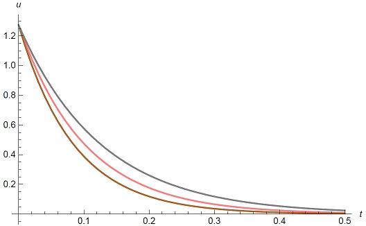
4.2 Temperature profiles in time

Setting x = x₀ in the approximate solution, we have

u(x,t)≈4u0πexp-q2π2t(ln(1+q))2. (42)

Figure 2 shows the plot of u versus t with u₀ = 1, x = x₀ for q = 0 (Red), q = 0.2 (Brown), and q = -0.2 (Gray).

Figure 2 Plot of u versus t with u₀ = 1, x = x₀ for q = 0 (Red), q = 0.2 (Brown), and q = -0.2 (Gray). 

5 q-deformed diffusion equation

The q-deformed diffusion equation has the same form as the 𝑞-deformed heat equation,

where u(x, t) denotes the concentration and D denotes diffusivity. Now let us impose the initial condition

Now let us introduce the 𝑞-deformed Fourier transform as

and the inverse q-deformed Fourier transform

From the definition of q-deformed Fourier transform, we know

Taking the q-deformed Fourier transform in Eq. (43) we get

which is solved as

Then we have

Thus we get

Now let us set

which gives

Then we have

From the convolution theorem we get

If we impose the initial condition

we have

From Eq. (57), the expectation value of x are

For a small q, we get

The variance is then given by

For a small q, we get

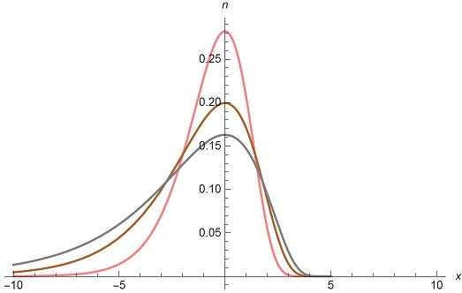
Figure 3 shows the plot of u(x, t) versus x with t = 1 and D = 1 for q = 0 (Pink), q = 0.2 (Brown) and q = -0.2 (Gray). We know that the graph is asymmetric unless q = 0. Thus Eq. (57) is the asymmetric normal distribution. Figure 4 shows the plot of u(x, t) versus x with q = 0.2 and D = 1 for t = 1 (Pink), t = 2 (Brown) and t = 3 (Gray). Figure 5 shows the plot of u(x, t) versus x with q = 0.2 and D = 1 for t = 1 (Pink), t = 2 (Brown) and t = 3 (Gray).

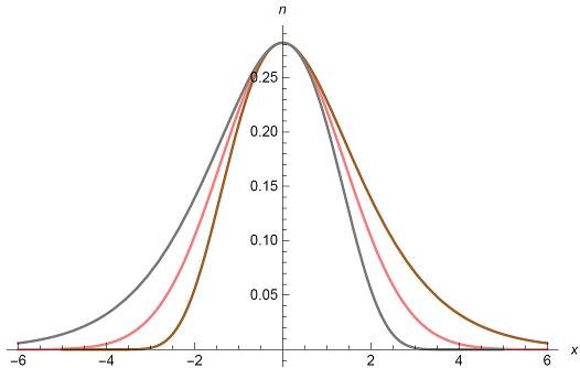
Figure 3 Plot of u(x, t) versus x with t = 1 and D = 1 for q = 0 (Pink), q = 0.2 (Brown) and q = -0.2 (Gray). 

Figure 4 Plot of u(x, t) versus x with q = 0.2 and D = 1 for t = 1 (Pink), t = 2 (Brown) and t = 3 (Gray). 

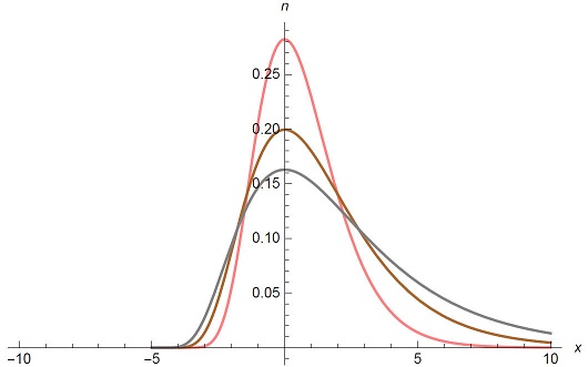
Figure 5 Plot of u(x, t) versus x with q = -0.2 and D = 1 for t = 1 (Pink), t = 2 (Brown) and t = 3 (Gray). 

6 Conclusion

In this paper we studied the q-deformed heat equation and q-deformed diffusion equation. From the fact that the ordinary heat equation was obtained by taking continuous limit in the discrete heat equation with a uniform space interval, we considered the discrete heat equation with a certain non-uniform space interval which was related to q-addition or q-subtraction appearing in the non-extensive thermodynamics. By taking the continuous limit, we obtained the q-deformed heat equation. We found that the q-deformed heat equation possessed the q-translation symmetry instead of the ordinary translation. We solved the q-deformed heat equation for a rod of length L. We discussed cooling of a rod from a constant initial temperature. We used the q-deformed Fourier transform to find the solution of the q-deformed diffusion equation. We found that the variance in x takes the form,

For a small q, we obtained

We found that the q-deformed diffusion process is asymmetric.

The q-addition and q-subtraction defined in the non-extensive thermodynamics was rarely used in the deformation of the space-time (q-deformed space time). The application to quantum mechanics was discussed in ^[20], application to mechanics was discussed in ^[25], and construction of q-lattice and q-Bloch theorem was discussed in ^[26].

Besides, we comment the connection of non-homogeneous media with the q-deformation of space briefly. It seems impossible to describe the general non-homogeneous media in an exact way without numerical study. Here, we adopted a special non-homogeneous media related to q-deformed space. Because asymmetry of the q-lattice, the graphs of temperature in the q-heat equation and concentration in the q-deformed equation became asymmetric, which had different feature for positive q and negative q, (See Fig. 1-5).

Finally, we compare the q-deformed diffusion equation with the diffusion model with the effective position dependent diffusion coefficient D(x) ^[27-29]. The diffusion equation with the effective position dependent diffusion coefficient D(x) was given in the form,

where w(x) denotes the variable cross section. Comparing Eq. (43) with Eq. (64), we know

Thus we know that the q-deformed diffusion equation is an example of the diffusion model with the effective position dependent diffusion coefficient.