


 text new page (beta)
 English (pdf)
 Article in xml format
 Article references
 Send this article by e-mail
 Cited by SciELO
  Similars in
SciELO
Similars in
SciELO 
 Permalink
1 Introduction
These days, circuit model-based quantum computers require some type of active error correction, because states in theoretically advantageous quantum algorithms acquire errors as they are prepared, manipulated by gates, and measured, reducing efficiency. For this reason, the characterization and correction of errors is of vital importance to obtain an acceptable result [2]. Although there are quantum error correction methods, as Fault-tolerant quantum error protocols [3], these are expensive from a computational point of view. In the current situation, i.e. a noisy intermediate-scale quantum era, it is important to characterize and analyze error models, for a possible future corrections.
The central idea of the article, is to use the isotropic index proposed in [1], that separates the model error into one part related to unitary deviation, due systematic errors, from another part which represents the loss of information. This last errors, due to decoherence, cannot be corrected without redundancy, while in principle systematic errors could be.
Two methods are proposed to model systematic errors. The first method determines the density matrix of the experimental output of a n qubit state, which requires about 4 n projective measurements (Quantum state tomography) and uses the isotropic index to find a unitary rotation, while the second method uses only 3n projective measurements. This last method is less general and works only for algorithms in which the output expected state, of each input basis state, is completely separable in all qubits.
With this intention, we analyze a particular algorithm: the Quantum Fourier Transform (QFT) [4], finding the unitary rotation that models the systematic error. The (QFT) is an important part of some quantum algorithms, such as the famous Shor’s factorization algorithm [5] and the quantum phase estimation algorithm [6]. However, the effect of noise on (QFT) is less studied. [7, 8].
This article is divided into three main sections. After the introduction, in Sec. 2, we present the Quantum Fourier Transform Algorithm (QFT), and its matrix model representation. In Sec. 3, we discuss both correction methods for general quantum algorithms. We explain how the unitary matrix model is determined for an n qubit state. Finally, in 4 we present, as an example, the experimental results of running the QFT algorithm for a two qubit system on IBM Q machine: ibmq_santiago, and some conclusions.
2 The quantum fourier transform algorithm
2.1 QFT Algorithm
The Fourier transform is used in a wide range of classical problems from signal processing to complexity theory. The QFT is the quantum generalization of the Discrete Fourier Transform (DFT) where the inputs are the amplitudes on a computational basis of a wave function. It is part of many quantum algorithms, most notably Shor’s factoring algorithm [5] which makes use of the QFT for period finding.
The classical DFT maps an input vector
where
Meanwhile the QFT acts on an input pure n-qubit quantum state x
where
where
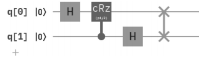
2.2 Circuit implementation
Experimental quantum computers nowadays generally use a small set of universal quantum gates in order to generate quantum circuits. The quantum IBM computer (IBM Q) is no exception and only works with certain quantum gates, which made translating the matrix in Eq. (4) to quantum gates an essential task.
As an example, for a two qubit state, the quantum gate representation of the algorithm requires a few basic gates: the Hadamard transform and a controlled rotation of angle
where Rz is
the QFT circuit
3 Systematic error model
3.1 Error model using the density matrix and the isotropic index
In order to model the systematic error, the first step is to reconstruct the resulting density matrix
For example, for any 2 qubit state its matrix
where
3.2 Isotropic index
The isotropic index is useful to separate the global loss of information, called weight
Considering the pure reference state
the double index is defined as:
where
where Fid is the fidelity between states [4], and
The misalignment takes values in the interval [-1,1], where 1 means the resulting state is completely aligned with the reference state
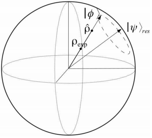
Consider now the state
it is always possible to obtain
In the particular case where
Unfortunately, generally the state
where A is the alignment index. These states can be graphically seen in Fig. 2.
In order to find
3.3 Error model using only 3n projection’s
Since determining the density matrix
Fortunately, in the case of the QFT algorithm, the theoretical output state for each input basis state is separable on all qubits. Although the mixed state
Once we have obtained the reduced density matrices of each qubit i, the eigenvector with the highest eigenvalue is extracted
Similarly to the previous method, the unitary rotation matrices are determined for each input basis state
As an example, the resulting unitary matrix for two qubits on IBM Q computer ibm_santiago, are shown in the next section and the results are compared to those of the first method.
4 Analyzing experimental results
The procedure will be explained for one of the basis input state of the algorithm
Running the QFT algorithm in IBM Q computer ibm_santiago, we estimate the resulting probabilities of measuring the projections in all basis. The mean values are obtained from 8192 shots for each projection, and shown in Tables I and II.
Table I Experimental results for the basis input state
| Basis | 0 | 1 |
|---|---|---|
| IX | 4103 | 4089 |
| IY | 7923 | 269 |
| IZ | 2230 | 1866 |
| XI | 162 | 3934 |
| YI | 2274 | 1822 |
| ZI | 4115 | 4077 |
Table II Experimental results for the basis input state
| Basis | 00 | 01 | 10 | 11 |
|---|---|---|---|---|
| XX | 202 | 120 | 3981 | 3889 |
| XY | 231 | 182 | 7266 | 513 |
| XZ | 158 | 147 | 4272 | 3615 |
| YX | 2299 | 2166 | 1874 | 1853 |
| YY | 4350 | 101 | 3587 | 154 |
| YZ | 2433 | 2016 | 2023 | 1720 |
| ZX | 2213 | 2052 | 2039 | 1888 |
| ZY | 4078 | 111 | 3875 | 128 |
| ZZ | 2204 | 1996 | 2167 | 1825 |
4.1 Experimental results with the isotropic index
Performing the QST on this data we obtained the experimental reconstructed density matrix for ibmq_santiago, which was deemed too large to fit this article.
The theoretical output state corresponding to input
Finally the unitary rotation matrix U
01 is calculated which maps the state
Table III Optimal pure state
|
|
|
|
|---|---|---|
| .565 | 0.559 | 0.586 |
| .450 + 0.031i | -0.480 - 0.006i | -0.026 - 0.453i |
| .485 - 0.010i | 0.534 + 0.021i | -0.498 |
| .488 - 0.063i | -0.414 + 0.015 | 0.015 + 0.450i |
This procedure was performed for the four resulting states, obtaining the four unitary transformations. Using two ancillary qubits, a unitary transformation U c is defined that controls which element of the unitary set should be applied, so that the model works for any input state. This model is shown in Fig. 3.
In order to model the decoherence, a total Depolarizing Chanel is applied on the theoretical state
is compared with the transformation of the experimental state under
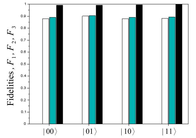
Finally in Table IV and as shown in Fig. 4, the results are compared. This comparison is done by calculating the fidelity in each step F 1, F2, F3 defined as:
where
Table IV Fidelities, Eq. (??) of the second method, using 4n projections, for ibm_santiago.
| Input state | F1 | F2 | F3 |
|---|---|---|---|
| |00〉 | 0.87940 | 0.88928 | 0.99213 |
| |01〉 | 0.90030 | 0.90551 | 0.99236 |
| |10〉 | 0.87870 | 0.88957 | 0.99553 |
| |11〉 | 0.88217 | 0.89308 | 0.99589 |
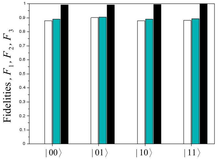
4.2 Experimental results Using only 3n projections
In contrast with the previous method, now we look for an estimate of the state
Finally the desired separable unitary rotation for each basis state
Table V Fidelities, Eq. (??) of second method, using 3n projections, for ibmq_santiago.
| Input state | F2 | F3 |
|---|---|---|
| |00〉 | 0.88471 | 0.98792 |
| |01〉 | 0.90541 | 0.99226 |
| |10〉 | 0.88857 | 0.99460 |
| |11〉 | 0.89133 | 0.99426 |

5 Conclusions
In this paper we have managed to study the performance of the Quantum Fourier Transform algorithm in a real quantum computer. The loss of information due decoherence effects, could be corrected by adding redundancy as in quantum correcting codes, but in general could be computationally expensive.
We propose two methods to model systematic errors: the first method uses the isotropic index that separates the loss of information, by decoherence, from the systematic error, that potentially could be correctable determining a unitary transformation that could correct any input state. The method needs to reconstruct the density matrix from 4 n measurements, and uses the alignment to determine the unitary correction matrix for each input basis state. Meanwhile, in the second method it is only necessary to measure 3n projections, taking advantage of the fact that the theoretical output of the QFT algorithm of each basis state, is separable in all qubits. The first method, although very expensive from a computational point of view, is more general and can be used to model systematic errors of any algorithm, the second can be only used for algorithms with separable output states as the QFT. Even though the theoretical output state of the QFT algorithm is separable, experimental errors can introduce some entanglement. Nonetheless, the experimental result is expected to be reasonably close to being separable for minor errors. As can be seen in Figs. 4 and 5, the results are very similar which seems to support this assumption.
As can be seen in these same figures, in actual IBM Q computers, the unitary errors are much less relevant than the decoherence errors. Nevertheless, this method could be used as calibration via software, using the U c matrix, once it is determined experimentally, regardless other methods are needed to correct decoherence error.
Even though this analysis shows correcting systematic errors at the current state of the art IBM Q computers is of minor importance, this models could be used to visualize (5) the weight of the different types of errors that affect quantum computation and could prove especially useful in educational contexts.

