1 Introduction

It is important to study the stability of the switched differential systems, since they are used in mathematical physics of many fields such as power systems, gravity, motor engine control, network control systems, constrained robotics, automotive engineering [^1-15]. One of the ways to examine the stability of switched systems is to study the dwell and average dwell time of the system.

We consider the linear switched system described by

where xt=xit is l dimensional vector, xit i=1,2,...,l are differentiable functions, P=1,2,…,N, Ap∈Cl×l,p∈P is matrix family, S=σ|σ:0,∞→P,σ switching signal. The amount of time passed between the consecutive switching events is called dwell time of system (1).

Let us give the definition of globally asymptotically stability (GAS) for the point x (t) = 0, which is the trivial solution and the equilibrium point of the switched system (1).

The trivial solution of the system (1) is GAS for a given switching signal σ if (1) is

If each subsystems are GAS then there exists a minimum dwell time that guarantees GAS of the system (1). For the system (1), let the following sets of switching signals be defined, where t _i ’s are successive switching time instants and Nσt is the number of switchings before time t:

Determination of the dwell or average dwell time is based on the calculation of the infimum of the numbers τ or τ¯ that makes the switched system GAS [^16-18].

There are many studies on the dwell and average dwell time for the GAS of the system (1) [^17-22]. These studies are generally used the eigenvalues of the coefficient matrices of the given system. It is well known that the eigenvalue problem is an ill-posed problem for non-symmetric matrices [^23-25]. Moreover, if a matrix has multiple eigenvalues, or is close to a matrix with multiple eigenvalues, then its Jordan normal form is very sensitive to perturbations. This ill conditioning makes it difficult to develop a robust numerical algorithm for the Jordan normal form. So, the Jordan normal form is usually avoided in numerical computations [^24-25].

A new method is proposed to determine the dwell and average dwell time without calculating the eigenvalue, in this paper. The proposed method depends on the κ(A) parameter, which shows the quality of the GAS of the systems of differential equations [^26-30]. “Dwell time" and “average dwell time" have not been studied depending on the κ(A) parameter yet, in the literature. Therefore, the results obtained in this study are new and original.

This paper is structured as follows: In Sec. 2, preliminaries are given. In Sec. 3, the dwell time and average dwell time for GAS are determined. Finally, numerical examples are given in Sec. 4.

2 Preliminaries

3 Determination of dwell time for GAS

Let us give the following theorem, which gives the upper bound of the solution of the system (1) to use determining the dwell time for GAS.

Theorem 2. The following equation is provided for the GAS matrix A_p (p = 1,2,…,N) where x(t) is the solution of the system (1):

where

Proof. Let the system (1) be given with GAS matrices A_p (p = 1,2,…,N). The solution of system (1) is expressed as

or

where x(0) = x₀ is the initial value of the system (1). By taking the norm of the solution (7) and applying the triangle inequality, the following inequality is obtained

If we use inequality (3), the upper bound of the solution is obtained as:

Therefore,

holds.

Theorem 3. The switched system (1) given by (4) is GAS for dwell times that provide the inequalityτ>ρ*D, wherew+i,j=(1/4)lnκ(Aσj)κ(Aσi), w-i,j=Aσj/κ(Aσj).

Proof. Suppose that σt has infinitely many switching. Because, when the switching signal has finitely switching, the system works in one of the subsystems after the last switching. Thus, since each subsystem is stable, the system (1) is GAS.

Let α be the weight of the walk W_n for the weight function wi,j=w+i,j-w-i,j in the switching graph D. Any walk with m nodes consists of cycles and a path with a maximum length of m - 1. Then it can be written as αn=α*n+∑i=2m‍αin. Here for i = 1,2,…, m, α_i (n), indicate the sum of the weights of all cycles with length i and α*n indicates the weight of the path. Since P is finite, α*n is bounded.

Let take us

and

So, we can write (6) by the equation

By taking τ≤ti-ti-1 and e-Aσn+1κ(Aσn+1)t-tn≤1 in (8), we obtain xt≤γeαnx0. Let us consider

for the walk W_n . Since τ>ρ*D by the assumption, the limit of α(n) as n approaches infinity is -∞. This means that upper bound (8) of the solution approaches zero as t→∞. Then, in the case of τ>ρ*D, system (1) is GAS.

Theorem 4. The switched system (1) given by (5) is GAS for average dwell times that provide the inequalityτ¯>μ*D/w*, wherew*=miniAσi/κ(Aσi).

Proof. Assume that σt has infinitely many switching, as in Theorem 3

Consider W_n as the walk for the weight function wi,j=w+i,j in the switching graph D. Similar to Theorem 3, for any walk with m nodes, it can be written as βn=β*n+∑i=2m‍βin. Here for i = 1,2,…, m, βin indicate the sum of the weights of all cycles with length i and β*n indicates the weight of the path. Let us take βn=∑i=1n‍lnκ(Aσi+1)κ(Aσi)1/4 and write the inequality (6) by the equation

using assumption w*=mini{Aσi/κ(Aσi)}.

If γ¯=γemaxWw+W, then the inequality (9) can be written as

Since βin are cycles for i = 1,2,…, m, we get ∑i=2m‍βin≤Nσtμ*D≤N0μ*D+tμ*D/τ¯.

Let define us γ¯¯=γ¯eN0μ*D and rewrite (10). So, the following inequality is obtained:

Since μ*D/τ¯-w*<0, the upper bound (10) of the solution approaches zero as t→∞. Then, system (1) is GAS.

4 Numerical examples

In this section, we give some numerical examples showing the efficiency of the results in Sec. 3.

Example 1. Let us consider the following system consisting three GAS subsystems:

Let D be the switching graph of the system (1) given inFig. 1.

Figure 1 Switching graphs of the Cauchy problem consisting of three subsystems with A₁, A₂, and A₃.  

Figure 2 State trajectory with τ=0.840262.  

For the graph D, the minimum dwell time calculated in Theorem 3 is obtained as τ=0.840262. For this minimum dwell time, if the system is switched for graph D, the solution curves given in the graph below are obtained.

Example 2. Let us consider the systems (1) with four GAS subsystems. For i∈{1,2,3,4}, let matrices A_i be given as follows

For systems (1), the switching graphs D1, D2 and D3 are given in Fig. 4.

Figure 3 State trajectory with x₁ a) and x₂ b) of system (11) .  

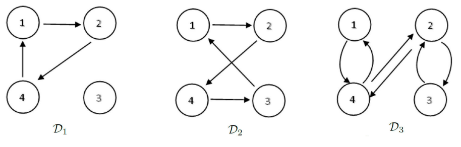
Figure 4 Switching graphs of the linear switched systems (1) consisting of four subsystems with A₁, A₂, A₃, and A₄.  

In Table I, computed dwell and average dwell times for the switching graphs Di    (i=1,2,3) are given.

As illustrated in Table I, for D1 switching graph, our dwell time (see Theorem 3) and average dwell time (see Theorem 4) values are better than the ones obtained by Karabacak [¹⁸]. Moreover, for D2 and D3 switching graphs, we are able to calculate dwell time from Theorem 3 and average dwell time from Theorem 4 although these values could not be calculated in [¹⁸] (because the A₃ is defective matrix). The values which we cannot calculate are denoted by the symbol * in Table I.

5 Conclusion

In this paper, dwell and average dwell time, which make differential equation systems (1) GAS, are calculated in terms of the κ(A) parameter without using eigenvalue. As far as we know, “dwell time" and “average dwell time" have not been studied depending on the κ(A) parameter in the literature. Therefore, the results obtained in this paper are new and original.

References

[1] I. Cantón, E. Campos-Cantón , S. Gonzalez-Bautista, R. Balderas-Navarro, Experimental multi-scroll attractor driven by switched systems, Rev. Mex. Fis., 63 (2017) 117. [ Links ]
[2] M. M. Elmetwally, N. D. Rao, Sensitivity Analysis in Power System Dynamic Stability Studies, IEEE Transactions on Power App. and Sys., PAS-91 (1972) 1692. [ Links ]
[3] D. Liberzon, Switching in Systems and Control, (Springer Science & Business Media, New York, 2012). [ Links ]
[4] S. Camazine, J. L. Deneubourg, N. R. Franks, J. Sneyd, E. Bonabeau, G. Theraulaz, Self-Organization in Biological Systems (Princeton University Press, Princeton, NJ, 2003). [ Links ]
[5] P. Holme, J. Saramäki, Temporal networks, Phys. Rep. 519 (2012) 97. [ Links ]
[6] D. Needleman, Z. Dogic, Active matter at the interface between materials science and cell biology, Nat. Rev. Mater. 2 (2017) 17048. [ Links ]
[7] O. Feinerman, I. Pinkoviezky, A. Gelblum, E. Fonio, N. S. Gov, The physics of cooperative transport in groups of ants, Nat. Phys. 14 (2018) 683. [ Links ]
[8] P. S. Churchland, T. J. Sejnowski, The Computational Brain (MIT Press, Cambridge, MA, 2016). [ Links ]
[9] C. K. Tse, M. Di Bernardo, Complex behavior in switching power converters, Proc. IEEE 90 (2002) 768. [ Links ]
[10] M. J. O’Mahony, D. Simeonidou, D. K. Hunter, A. Tzanakaki, The application of optical packet switching in future communication networks, IEEE Commun. Mag. 39 (2001) 128. [ Links ]
[11] S. Solmaz, R. Shorten, K. Wulff, F. O’Cairbre, A design methodology for switched discrete time linear systems with applications to automotive roll dynamics control, Automatica 44 (2008) 2358. [ Links ]
[12] A. Balluchi, M. D. Benedetto, C. Pinello, C. Rossi, A. Sangiovanni-Vincentelli, Cut-off in Engine Control: A Hybrid System Approach, in Proceedings of the 36th IEEE Conference on Decision and Control, (1997) 4720. [ Links ]
[13] B. E. Bishop, M. W. Spong, Control of Redundant Manipulators Using Logic-Based Switching, in Proceedings of the 36th IEEE Conference on Decision and Control, (1998) 16. [ Links ]
[14] W. Zhang, M. S. Branicky, S. M. Phillips, Stability of Networked Control Systems, IEEE Control Systems Magazine, 21 (1998) 84. [ Links ]
[15] D. Z. Chen, Y. J. Guo, Advances on Switched Systems, Control Theory and Applications, 22 (2005) 954. [ Links ]
[16] A. Kundu, D. Chatterjee, Stabilizing switching signals for switched systems, IEEE Transactions on Automatic Control 60 (2015) 882. [ Links ]
[17] J. P. Hespanha, A. S. Morse, Stability of switched systems with average dwell-time, in: Proc. of the 38th Conf. on Decision and Control, (1999) 2655. [ Links ]
[18] Ö. Karabacak, Dwell time and average dwell time methods based on the cycle ratio of the switching graph, Systems Control Lett. 62 (2013) 1032. [ Links ]
[19] S. Morse, Supervisory control of families of linear set-point conrollers-part 1:exact matching, IEEE Trans. Autom. Control, 41 (1996) 1413. [ Links ]
[20] J. C. Geromel, P. Colaneri, Stability and stabilization of continuous-time switched linear systems, SIAM J. Control Optim. 45 (2006) 1915. [ Links ]
[21] P. Colaneri, J. C. Geromel, A. Astolfi, Stabilization of continuous-time switched nonlinear systems, Systems Control Lett. 57 (2008) 95. [ Links ]
[22] Ö. Karabacak, N. S. Şengör, A dwell time approach to the stability of switched linear systems based on the distance between eigenvector sets, Inter. J. Syst. Sci. 40 (2009) 845. [ Links ]
[23] J. H. Wilkinson, The Algebraic Eigenvalue Problem (Clarendom Press, Oxford, 1965). [ Links ]
[24] G. H. Golub, C. F. V. Loan, Matrix Computations (Johns Hopkins University Press, Baltimore, 2013). [ Links ]
[25] G. H. Golub, J. H. Wilkinson, Ill-conditioned eigensystems and the computation of the Jordan canonical form, SIAM Rev. 18 (1976) 578. [ Links ]
[26] A. Ya. Bulgakov, An effectively calculable parameter for the stability quality of systems of linear differential equations with constant coefficients, Siberian Math. J. 21 (1980) 339. [ Links ]
[27] A. Ya. Bulgakov, Matrix Computations with Guaranteed Accuracy in Stability Theory (Selçuk University The Research Center of Applied Mathematics, Konya, 1995). [ Links ]
[28] S. K. Godunov, Ordinary Differential Equations with Constant Coefficients (Translations of Mathematical Monographs, American Mathematical Society, Providence, 1997) [ Links ]
[29] H. Bulgak, Pseudoeigenvalues, spectral portrait of a matrix and their connections with different criteria of stability, in Error Control and Adaptivity in Scientific Computing, eds. H. Bulgak and C. Zenger, NATO Science Series, Series C: Mathematical and Physical Sciences, Vol. 536 (Kluwer Academic Publishers, Dordrecht, 1999), pp. 95-124. [ Links ]
[30] A. Duman, K. Aydın, Sensitivity of Hurwitz stability of linear differential equation systems with constant coefficients, Int. J. Geom. Methods Mod. Phys. 14 (2017) 1750084. [ Links ]
[31] J. P. Padrón, J. P. P. Padrón, Trajectory tracking error using fractional order time-delay recurrent neural networks using Krasovskii-Lur’e functional for Chua’s circuit via inverse optimal control, Rev. Mex. Fis. 66 (2020) 98. [ Links ]
[32] A. Dasdan, R.K. Gupta, Faster maximum and minimum mean cycle algorithms for system-performance analysis, IEEE T. Comput. Aid. D. 17 (1998) 889. [ Links ]
[33] A. Dasdan, Experimental analysis of the fastest optimum cycle ratio and mean algorithms, ACM Trans. Des. Autom. Electron. Syst. 9 (2004) 385. [ Links ]
Received: August 26, 2021; Accepted: September 23, 2021
Creative Commons License This is an open-access article distributed under the terms of the Creative Commons Attribution License