


 text new page (beta)
 English (pdf)
 Article in xml format
 Article references
 Send this article by e-mail
 Cited by SciELO
  Similars in
SciELO
Similars in
SciELO 
 Permalink
1 Introduction
Magnetohydrodynamics (MHD) is concerned with the interaction of flowing fluids and magnetic fields. The fluid in question must be electrically conducting and non-ferromagnetic such as metal-based fluids, plasmas and electrolytes [1]. Theoretical models of MHD flows are formulated by coupling the Navier-Stokes equations and Maxwell’s equations, both systems of equations couple via the Lorentz force. Numerous studies have already been conducted on MHD flows for industrial applications such as heat sinks in nuclear reactors, pumps, batteries and levitating liquid metals.
On the interaction between liquid metal and magnetic fields, numerous experimental investigations of metal fluids flowing through a channel to which an artificial external magnetic field is applied have been performed [2, 3, 4]. A fluid electrically conducting that flows trough a channel in the presence of an external magnetic field produced by a magnet suffers a magnetic braking in it’s momentum by Lorentz force, i.e., induced electrically currents are produced inside the entire fluid flow due the relative movement to the applied magnetic field, thus the Lorentz force results in an induced magnetic force in the opposite direction of fluid flow, thereby causing the fluid to slow its motion. This effect has also been observed experimentally in the case of a rising single helium bubble in a metal liquid environment like mercury under vertical magnetic field [5], which demonstrate that the rise velocity of helium bubble decreases monotonically with the increase of the magnetic field. The latter results were confirmed with numerical simulations by means of two-phase interface treatment [6, 7].
In particular, the dynamics of liquid metal jets/drops is important, for example, in the development of alternative energy sources such as new plasma-based fusion reactors like the Tokamak [8], or the development of revolutionary three-dimensional printing based on liquid metal generated by melting which is printed using an ink-jetting process [9]. Furthermore, studies of exoplanet atmospheres such as those of the giant exoplanet WASP-76b [10] demonstrate the possibility of molten iron raining as droplets. It is suspected that this rainfall is affected by induced MHD effects.
The effect on the motion of a liquid metal drop falling in presence of a magnetic field was studied first by [11]. The authors computed the force promoted by the interaction of the induced electric currents generated into the drop and the applied magnetic field. They concluded that no matter the sign of the magnetic field gradient, the electromagnetic force is always in the opposite direction of the drop motion, acting as an electromagnetic drag. More recently, the study of a falling metal drop was performed by a numerical simulation [12], where a drop fell into a metal liquid layer in the presence of imposed vertical magnetic field, such results revealed an interesting behaviour on metal liquid layer for a strong magnetic field, spreading was substantially reduced and a swelling of free surface after collision were observed. An interesting investigation is presented in [13], where numerical simulations were performed of a falling droplet in the presence of a positive and negative magnetic field gradient.
In contrast to previous works, we present a theoretical and experimental study of a falling metal drop under the effect of a perpendicular magnetic field. The experimental set-up is rather simple and useful which does not require expensive high speed cameras since it is a liquid-liquid phase experiment. Additionally, in the numerical simulations a real distribution of the magnetic field was used in order to compare the phenomenon with the experimental observations.
2 Experimental procedure
The experiment set up consist of a liquid metal drop falling in a Hele-Shaw cell. The cell consist of two sheets of tempered glass glued to an O-ring and kept fixed with aluminium forceps. The cell’s dimensions are 230 mm long 110 mm width and a separation between sheets of 2.5 mm. The cell is vertically placed and is open in the upper side, see Fig. 1. A rectangular parallelepiped Neodynium magnet with a side length of 50.8 mm, height of 25.4 mm is placed in the geometrical center outside the cell. The z - axis of the magnet is perpendicular to the cell. The perpendicular component of the magnetic field was measured with a Teslameter F.W. BELL, model 4048. The maximum strength of the magnetic field at the cell’s centre is 0.22 T, as seen in Fig. 2.
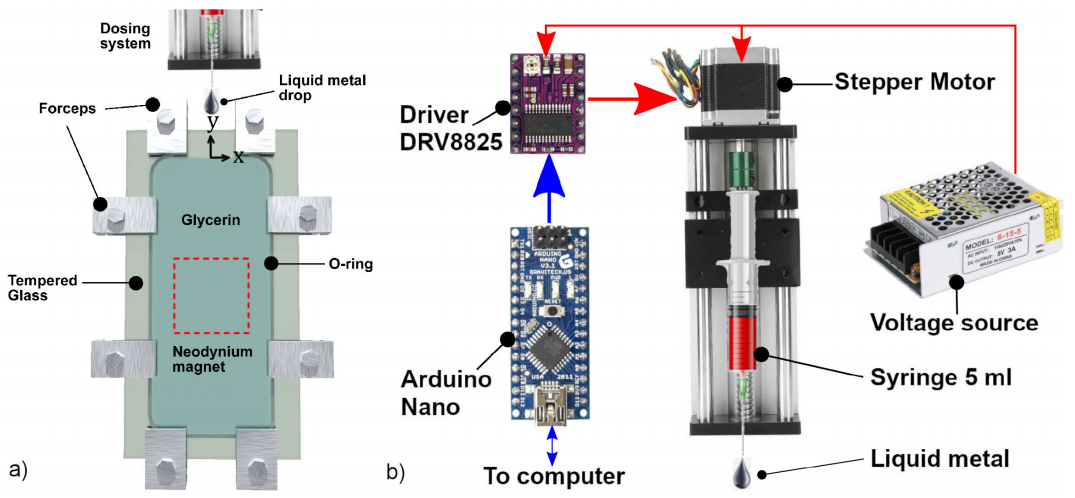
Figure 1 Sketch of the experimental set-up, not drawn to scale. a) Hele-Shaw cell. The flow promoted by falling drop is visualized in the x-y plane thorough the PIV technique. b) Diagram of the liquid metal droplet dosing system and its components. Blue lines indicate the flow of control signals and red lines indicate the flow of electrical current.
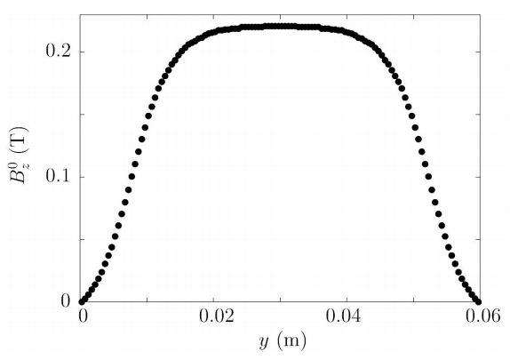
Figure 2 Perpendicular component
The formation of liquid metal drops was carried out by automating a 5 ml syringe. It was manually filled with liquid metal during testing, later it is placed on a screw linear actuator (six centimeters of travel), the which implements a stepper motor (nema 17) to linearly move the plunger of the syringe. The volume of the drop (V = 0.022 ml) is controlled by varying the angular velocity and the number of steps of the motor, for this purpose, an Arduino Nano microcontroller and the DRV8825 driver are used. The latter generated liquid metal drops with diameter d = 3.4 mm. Figure 1b) shows the components used for dosing drops of liquid metal. The measures of the cell were calculated so that its boundaries are sufficiently far away from the metal drop.
In order to obtain low Reynolds flows, the cell was filled with glycerin rather than air, thus the drag is increased. The working fluids are at room temperature (20° C). The drop is an eutectic alloy of Gallium, Indium and Tin (GaInSn) that is liquid at room temperature; its mass density, kinematic viscosity and electrical conductivity are ρ1 = 6360 Kg/m3, v = 3.4 × 10⁻⁷ m2/s and
3 Theoretical model
3.1 Numerical solution
Consider a two dimensional fluid composed by two-immiscible fluids (a continuous phase and a liquid metal droplet) in presence of the acceleration of gravity. The distribution of the magnetic field is modeled as in [16] that corresponds to the distribution found experimentally, as seen in Fig. 2. The drop falls due to its weight and the continuous phase is displaced by the moving drop. The surface tension between the two fluids is taken into account in the model, and the geometry of the interface is calculated by considering the normal and tangential stresses that arise due to the interaction of the drops and the surrounding liquid. Due to the complexity of the problem, it was approached numerically by a finite volume/front-tracking method where a single set of conservation equations [17] are solved for the entire domain, including the liquid metal drop and the continuous phase. The details of the numerical implementation can be found in [18]. The equations that describe the motion of the drops and the surrounding are mass and momentum conservation coupled with electromagnetic equations for computing the induced magnetic field with the low magnetic Reynolds number approximation [1, 19]. Considering that the two fluids are incompressible, the mass conservation is given by:
where u is the fluid velocity. The momentum conservation equation is written in a form that includes the different fluids and the surface tension force:
The pressure is denoted by p, μ is the dynamic viscosity, g is the gravity vector,
where
Once the induced magnetic field is calculated, the induced electric current can be found as:
where
3.2 Analytical solution
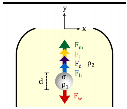
Following the approach for the dynamics a spherical particle to a one-dimensional flow by Morsi[20], a simple approach of the drop dynamics is the balance of the forces (as seen in Fig. 3) which act on the liquid metal drop
where F d is the drag, F b is the buoyancy, F m is the induced magnetic force, F f is the friction doe to the walls of the cell and F w is the weight. The latter forces can be mathematically expressed as
where m is the mass of the metal drop, v is the velocity, t denotes time, C
D
is the drag coefficient, A is the superficial area of the drop, V is the volume and g is the gravity acceleration,
The total magnetic force (or Lorentz force) in the drop due to the induced currents is
Considering that only the component of the applied magnetic field normal to the plane of motion is relevant,
considering that the drop only moves in the negative y- direction and the induced magnetic field only depends the vertical direction, it goes as
By integration by parts and assuming low acceleration
From Ampére’s law (Eq. (5))
Consequently, the magnetic force (
where d is the diameter of the drop. By scaling the velocity and time with
where the dimensionless parameters Re, Ha, K and G denotes the Reynolds number, Hartmann number and the dimensionless friction and gravity acceleration, respectively, which are defined as
where v is the kinematic viscosity. We note that, the behavior of MHD flows can be characterized by the Hartmann number, that represent a relation between magnetic with respect the viscous forces. The solution to the Eq. (14) is
where the initial condition is zero. The parameters a, b and c are defined as
The drag coefficient C D can be obtained from [20]
Finally, if the solution for the velocity ((16)) is integrated, we can obtain the position of the drop as a function of time
We must note that, this is an idealized model that can only be compared with the experiments in a qualitative level as will be shown in next section.
4 Results
Figure 4 show the experimental snapshots of the falling metal drop (first row) along with the vector fields (second row) for different time instants. The vector fields allows to easily identify the flow structure as the metal drop falls surrounded with the glycerin, namely, a dipole vortex. Moreover, the vector fields allow us also to identify the direction of the flow and its magnitude.
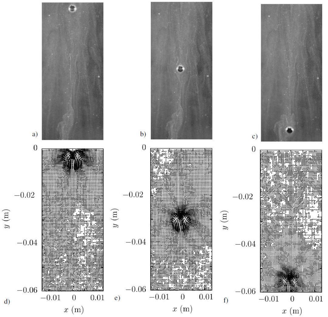
Figure 4 First row: Snapshots of the falling metal drop for Ha = 0 at different time instants t = 0.5 s, t = 3.5 s and t = 6.8 s. b) Second row: PIV velocity fields of the drop for the latter time instants. Experimental observations.
The tracking of the metal drop allows to obtain the position of the drop in every frame of the recorded video, Fig. 5 shows the position of the drop as a function of time. We can observe that for the hydrodynamics case, that is Ha = 0, the drop traverses the domain presented in Fig. 5a) (l = 0.06 m) in t = 7.3 s, meanwhile it lasts t = 9.1 s when the induced magnetic effects are present, in this case the Hartmann number is Ha = 0. The above shows the braking effect on the drop due to the presence of the magnetic field gradient. Because the relative motion of the droplet with respect to the magnetic field, induced currents are generated. The interaction of the induced currents and the applied magnetic field produce a Lorentz force in the metal drop. This electromagnetic force is produced in the opposite direction of acceleration of gravity and as a consequence slows down the motion of the drop. From the latter data, we can calculate a mean velocity: v m = -7.7 ( 10-3 m/s and v m = -6.2 ( 10-3 m/s, for Ha = 0 is and Ha = 30, respectively.
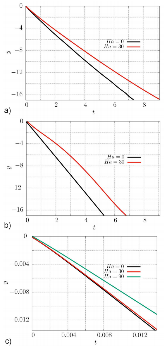
Figure 5 Vertical position y of the metal drop as a function of time t. a) Experimental data. b) Numerical simulation. c) Analytical solution from (19).
The Reynolds number for the experiments is
Simulations are able to give a deep insight in the drop motion and flow generated function of time. In Fig. 6, the velocity of the metal drop as function of time is presented computed from the numerical simulations. The vertical lines mark the instants of time in which the metal drop enters and leaves the magnetic field. Additionally, the instant where the drop is in the area where the field produced by the magnet permanently is maximum is also marked. As it can be observed, once the metal drop enters in the magnetic field, the extra drag promoted by the Lorentz force causes a deceleration of the drop, in this zone a high magnetic field gradient promotes that the Lorentz force be intense. Once the drop leaves the magnetic field, it accelerates until reaches the approximately the same velocity of the Ha = 0 case. The interaction found is consistent with the analytical and numerical results reported by [11, 13], respectively, but in this case, the effect of the Lorentz force on the metal drop dynamics is shown for a case that can be reproduced by an experiment using an approximation of a real magnetic field distribution generated for a given permanent magnet.
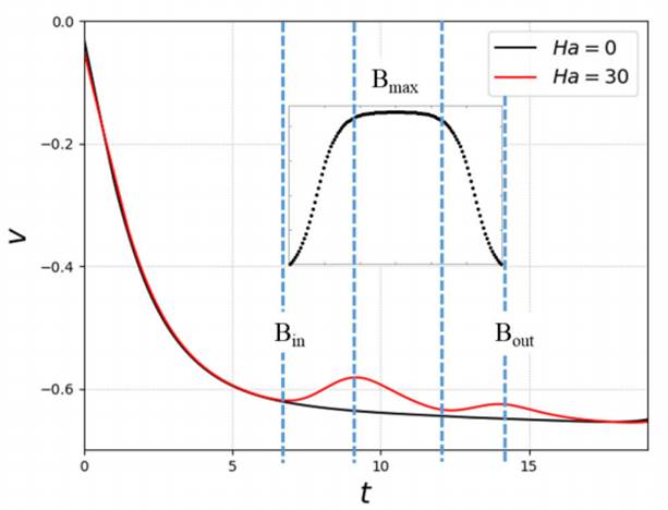
Figure 7, the falling metal drop and the velocity field are shown at the same instant of time for Ha = 0 and Ha = 30. For both cases the flow formed around the drop is a dipole vortex, as seen in the experimental PIV results (second row in Fig. 4). Due the low Reynolds number, for both simulations, the metal drop follows an approximately straight path along its fall, which matches with the one-dimensional flow assumption in the analytic solution. In the case of Ha = 0, the drop tends to remain with a circular shape during all the trajectory, while for Ha = 30, the drop shape changes to an ellipse due to the Lorentz force promoted by the interaction of the induced current and the applied magnetic field. As it was commented, the Lorentz force acts in the opposite direction of the gravity acceleration in the zones where the applied magnetic field gradient is intense, and this force acts as a brake on the motion of the drop.
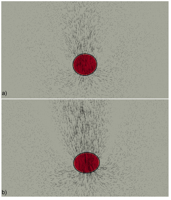
Figure 7 Velocity field (black arrows) and falling metal drop (red color). a) Ha = 0. b) Ha = 30. Numerical simulations.
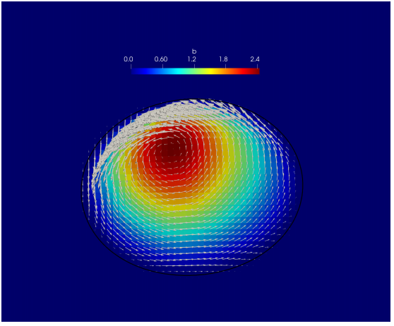
In order to explain how the Lorentz force produces a braking effect on the drop’s motion, the electric current density vector and contours of the induced magnetic fields inside the metal drop are shown in Fig. 8. The induced current manly points in the negative x—direction, while the magnetic field is in the z-direction, thus the magnetic force is in the y-direction which is contrary to the drop’s motion. As can be appreciated, due to the deformation and the internal flow inside the drop, the electric currents form non-axisymmetric closed loops along polar axis. The small deviation from a rectilinear path due to the Reynolds number reached by the drop promotes that it does not pass through out the central line of the permanent magnet making the electric currents and induced magnetic field not symmetric with respect to the longitudinal axis of the metal drop. The symmetric case for the induced currents occurs the drop is a non-deformable solid [11].
5 Concluding remarks
The falling metal drop falling in a localized magnetic field has been studied theoretically and experimentally in the laminar regime (Re = 76). The metal drop falling in glycerin was observed experimentally through PIV and image tracking. An analytical solution for the falling drop under several body forces was derived. A numerical solution based on the so-called front-tracking method for the incompressible Navier-Stokes equations was implemented. The simulations were performed for a size similar to the experimental Hele-Shaw cell in order to analyze the complete trajectory of the metal drop, including the zone where it interacts with the applied magnetic field. It was found that at the zones in which is a intense magnetic field gradient, the drop decelerates due to the generated Lorentz force that counteracts the gravity acceleration, however, in the zone where the applied magnetic field is approximately constant, there is no electromagnetic interaction between the metal drop and the permanent magnet.The flow and electrical current were also analyzed and it was found that at the presented flow conditions, the Lorentz force tends to deform the drop, also, the unbalance in the pressure gradient promoted by the reached Reynolds number deviates the drop from a rectilinear path and as a consequence, the induced currents and magnetic field inside the drop are non symmetric with respect to the longitudinal axis of the metal drop. The analytical and numerical solutions represent qualitatively the experimental problem. To the best of our knowledge, this is the first reported experimental study for liquid metal drops falling in the presence of a perpendicular non-uniform magnetic field.

