1. Introduction

An important and notable feature of solutions to Einstein theory of gravity, such as Schwarzchild spacetime or the cosmological Friedmann-Lemaître-Robertson-Walker solution, is that they all have apparent singularities. The question was, what would be their physical implications? It was Raychaudhuri who tried to investigate these solutions in both cosmological ^[1] and gravitational contexts ^[1]. Later, in 1955, he proposed his famous equations ^[3] which are known as Raychaudhuri equations.

These equations appeared to be of great importance in describing gravitational focusing and spacetime singularities, which are essentially explained by the so-called Focusing Theorems. Assuming Einstein equations and using energy conditions, it is established that time-like and null geodesics, if they are initially converging, they will focus until reaching zero size in a finite time. One of the most important notions about singularities, as pointed out by Landau and Lifshitz ^[7], is that a singularity would always imply focusing of geodesics, while focusing itself does not imply a singularity. Therefore in their work, the concept of geodesic focusing (although not explicitly stated the same) was worked out. However, they did not introduce shear and rotation, which are inseparable ingredients of Raychaudhuri equations.

Ever since the equations were published, they have been discussed and analyzed in numerous frameworks of general relativity, quantum field theory, string theory and relativistic cosmology. One should note that the concept of a singularity was first defined in seminal works of Penrose and Hawking ^[4-^6]. Therefore, it was only then that Raychaudhuri equations received their deserved acclaim.

In addition to general relativity, the Raychaudhuri equations have also been discussed in the context of alternative theories of gravity, such as f(R) theories ^[8]. In this paper as well, we consider characteristics of time-like flows in an alternative theory of gravity which as well has cosmological implications, namely, the Weyl theory of gravity. The paper is organized as follows: in Sec. 2 we briefly introduce the Raychaudhuri equations and its kinematical parameters; in Sec. 3 we mention the Weyl field equations and obtain the kinematical evolution of time-like radial and rotational geodesic flows, and see how they behave by plotting the congruences of the integral curves. Finally in Sec. 4, we summarize the results.

2. Raychaudhuri Equations

As it was mentioned, the Raychaudhuri equations are evolution equations for expansion, shear and rotation of a time-like geodesic congruence of integral curves, which is indeed pure geometrical and therefore, are independent of reference frames of Einstein equations. Being parametrized in terms of the affine parameter of the geodesics, τ, these in 4-dimensional spacetimes are written as follows ^[9]:

In Eqs. (1) to (3), Θ, σμν and ωμν are respectively the scalar expansion, the symmetric trace-less shear tensor and the anti-symmetric rotation tensor. Moreover, σ2=σμνσμν, ω2=ωμνωμν and Cλνμρ are the Weyl conformal tensor. In Eq. (1), vμ denotes the tangential vector field on the geodesics and hμν in Eqs. (2) and (3) are the projection tensor which for time-like curves and is defined by:

Generally speaking, the Raychaudhuri equations deal with the kinematics of flows which are generated by vector fields. Such flows are indeed congruences of integral curves which may or may not be geodesics. Actually, in the context of these equations, we are interested in the evolution of the kinematical characteristics of the so-called flows, not the origin of them. These characteristics which are contained in the Raychaudhuri equations, may constitute one equation like ^[10]:

in which the trace-less symmetric part is defined as:

Also, the scalar trace is and the anti-symmetric part are:

Geometrically, these quantities are related to a cross-sectional area, which encloses a definite number of integral curves and is orthogonal to them. Moving along the flow lines, this area may isotropically changes its size or being sheared or twisted, however, it still holds the same number of flow lines. There are some analogies with elastic deformations which are discussed in Ref. ^[11]. Also, one can find explicit discussions on these quantities in Refs.^[12,^13].

Here we should note that the Raychaudhuri’s equations may be essentially regarded as identities, which become equations when they are, for example, used in spacetimes defined by Einstein field equations.

Moreover, these equations are of first order and non-linear. Also, the expansion equation in Eq. ([1]), is the same as Riccati equation in a mathematical point of view ^[14,^15]. The expansion is indeed the rate of change of the cross-sectional area, which is orthogonal to the geodesic bundle.

In the next section, we will find the mentioned kinematical characteristics, for curve bundles on a definite spacetime background.

3. Time-like Geodesic Congruences in Weyl Gravity

The Weyl theory of gravity has had an interesting background and had received a great deal of attention from those who believe that the dark matter/dark energy scenarios, could be well-treated by altering general theory of relativity. This became more elaborated after arguing that the extraordinary behavior of the galactic rotation curves, could be extracted from Weyl gravity as a natural consequence of its vacuum solutions ^[16-^18]. There were subsequently more attempts to make relations between the theory’s anticipations and observational evidences ^[19-^21] and as the main course, proposing gravitational alternatives to dark matter/dark energy ^[23-^25]. Some good information about this 4th order theory of gravity can be found in Ref. ^[22] . Another important feature of the Weyl theory of gravity, is its conformal invariance which, as it is stated in the literature, could be considered as a tool of unification with the standard model by creating the desired mass during the symmetry breaking ^[26].

The Weyl theory of gravity, is a theory of 4th order with respect to the metric. Weyl gravity is characterized by the Bach action:

where C2=CμνρλCμνρλ is the Weyl invariant and α is a coupling constant. The action in Eq. (9) in principle, could be rewritten as:

from which, using the total divergency of the Gauss-Bonnet term -g RμνρλRμνρλ-4RμνRμν+R2, we have:

Varying Eq. (11) with respect to gμν, one obtains the Bach tensor as ^[16]:

Accordingly, the Weyl field equations read as:

where Tμν is the matter/energy tensor. Also the vacuum field equations (Wμν=0) have been explicitly solved. The solution constructs a spherically symmetric spacetime defined by the line element ^[16]:

in which:

This solution has three important constants, β,γ and k, by which the Schwarzschild-de Sitter metric could be regenerated. Also γ and k are respectively related to the dark matter and dark energy constituents of the cosmic fluid. Now let us inspect how time-like flows evolve in the spacetime defined in Eq. (14). To do this, we separately consider radial and rotational flows, and obtain the kinematical parameters in the Raychaudhuri equations.

3.1 Radial Flows

Some features of pure radial time-like flows has been discussed in Ref. ^[27]. Firstly, for the spacetime coordinates on a parametric integral curve:

xμ=t(τ),r(τ),θ(τ),ϕ(τ), (16)

we define the velocity 4-vector field:

vμ=ṫ(τ),ṙ(τ),θ̇(τ),ϕ̇(τ), (17)

which is supposed to be tangential to any integral curve inthe spacetime and for time-like congruences, one must have vμvμ=-1. Also ẋμ denotes d/dτ. To have purely radial flows on the equatorial plane, we take θ=π/2 and ϕ̇=0. Therefore, for such flows in the spacetime defined in Eqs. (14) and (15), the time-like condition is:

gμνvμvν=-1, (18)

and the geodesic equations:

v̇μ+Γμνλvνvλ=0, (19)

are respectively:

rṙ2β(3βγ-2)-kr3+γr2-3βγr+r+ṫ2β+kr3-γ3β2+r2-3βr-r+rr=0, (20)

ṙṫβ(3βγ-2)+2kr3-γr2rβ(2-3βγ)+kr3-γr2+r(3βγ-1)+ẗ=0, (21)

β(3βγ-2)+2kr3-γr2ṫ2β(3βγ-2)-kr3+γr2-3βγr+r2-r2ṙ22r3β(2-3βγ)+kr3-γr2+r(3βγ-1)+r̈=0, (22)

Integrating Eq. (21) we obtain:

ṫ=r-3β2γ+2β+kr3-γr2+3βγr-r, (23)

using which in Eq. (20), gives

ṙ=±-3β2γ+2β+kr3+3βγr-γr2r. (24)

Taking the positive part, the tangential vector field in Eq. (17) for pure radial flows becomes:

vμ=(r-3β2γ+2β+kr3-γr2+3βγr-r,-3β2γ+2β+kr3+3βγr-γr2r,0,0). (25)

The flows, which are formed by this vector field, are expanding by the following factor which is obtained by use of Eq. (7):

Θ=6kr3-5γr2+3β(-3βγ+4γr+2)2r3/2kr3-γr2+β(-3βγ+3γr+2). (26)

The vector field in Eq. (25) is orthogonal to the hypersurface of the field crests. Therefore, it is of zero rotation ^[11]. However, the shear tensor is non-zero. From Eqs. (4), (6) and (26), we have:

σtt=9β2γ+γr2-6β(γr+1)-3β2γ+kr3-γr2+β(3γr+2)3r5/2 (27a)

σtt=σrt=-9β2γ+γr2-6β(γr+1)3rβ(2-3βγ)+kr3-γr2+r(3βγ-1), (27b)

σtt=r9β2γ+γr2-6β(γr+1)3-3β2γ+kr3-γr2+β(3γr+2)β(3βγ-2)-kr3+γr2-3βγr+r2, (27c)

σtt=σϕϕ=-r9β2γ+γr2-6β(γr+1)6-3β2γ+kr3-γr2+β(3γr+2). (27d)

To obtain a pictorial viewpoint of how radial flows will behave in a Weyl field, we should find an expression for r(τ). Using Eq. (23), the geodesic equation in Eq. (22) gives:

r̈-ṙ2-1β(3βγ-2)+2kr3-γr22rβ(2-3βγ)+kr3-γr2+r(3βγ-1)=0. (28)

Unfortunately, this is a non-linear second order equation. Even the first order equation in Eq. (24) could not be explicitly solved. Therefore, we consider a simpler case of γ=0 which is in accordance to the de Sitter solution. In this case, Eq. (24) results in:

r(τ)=±e-k(c+τ)e3k(c+τ)-2βk2/322/3k2/3, (29)

with:

c=13ln2k3r032β+kr03+k2r03+βkk,

where r0 is the point of closest approach. The radial flows are shown in Fig. 1. One can note how the expansion will make cross-sectional area to change its size.

FIGURE 1 The purely radial flows in a Weyl field with γ = 0. 

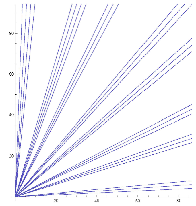
3.1.1 Focusing

If spacetime singularities are concerned, Eq. (1) for the expansion receives the most central attention. As it was shown above (and also in Fig. 1), the expansion changes the cross-sectional area along the geodesic bundle. It is noted that, if the expansion approaches the negative infinity, the congruences will converge, whereas they diverge if the expansion goes to positive infinity. The convergence, is what we regard as the focusing of the geodesic bundles toward the singularities. However, to clarify whether any convergence occurs for a peculiar flow, one should examine the expansion equation. It has been put in the literature that, convergence occurs if:

Rμνvμvν+σ2-ω2≥0, (30)

or equivalently,

dΘdτ+13Θ2≤0. (31)

Therefore, one can observe that shear acts in favor of convergence, while rotation opposes it. However, for zero rotations the condition in Eq. (30) reduces to ^[10]:

Rμνvμvν≥0. (32)

Now, for the zero-rotational flow defined by the vector field in Eq. (25), the condition in Eq. (32) gives:

γr-3k≥0. (33)

This provides us a maximum for r according to which, one must have r≤(γ/3k). We should note that the metric potential in Eq. (15), includes a Newtonian 1/r term, which is dominant at small distances. Increasing r, it would be the term γr as the dominant one. Such distances are about galactic scales. For a typical galaxy of radius r∼10 kpc, γ is of order 10-26 m-1 and at cosmological distances, the coefficient k in the term kr2 is of the greatest importance, which for a universe of constant curvature, may be regarded as the cosmological parameter of order 10-43 m-2. ^[28,^29]Therefore, if galactic scales are of interest, Eq. (30) implies that for r≲3.3×1016 m we may expect the convergence of the flow.

3.2 Rotational Flows

Pure rotational flows in the equatorial plane, could be obtained by letting θ=π/2 and r=const., according to the vector field in Eq. (17). Hence, the time-like condition in Eq. (18) and the geodesic Eqs. (19) are respectively:

t˙2(β(2-3βγ)+kr3-γr2+r(3βγ-1))+r3ϕ˙2+r=0, (34)

i¨=0 (35)

t˙2(β(3βγ-2)+2kr3-γr2)+2r3ϕ˙2=0, (36)

Φ¨=0 (37)

Equation (35) implies ṫ=1. Applying this to Eq. (34) gives:

ϕ̇=±3β2γ-2β-kr3+γr2-3βγrr3/2. (38)

Therefore, the tangential vector field can be written as:

vμ=1,0,0,3β2γ-2β-kr3+γr2-3βγrr3/2. (39)

Together with Eq. (7), one can see that Θ=0, implying that the flows which are formed by Eq. (39), are free of expansion. Therefore, we can not expect any focusing for this rotational flow, since the cross-sectional area does not change. Also the non-zero components of the shear tensor would be:

σrϕ=σϕr=-9β2γ-γr2+6β(γr+1)4r3β2γ-kr3+γr2-β(3γr+2). (40)

Moreover, using Eq. (8), one can obtain the rotation of the flow, which is characterized by the following non-zero components of the anti-symmetric part of the Raychaudhuri kinematical parameters:

ωtr=-ωrt=kr--3β2γ+2β+γr22r2, (41a)

ωrϕ=-ωϕr=-3β2γ+4kr3-3γr2+β(6γr+2)4r3β2γ-kr3+γr2-β(3γr+2). (41b)

The constant radial distance can be obtained from Eqs. (36) and (38). We have:

r=3βγ±6βγ. (42)

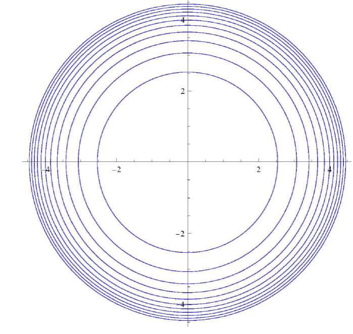
According to this, the pure rotational flow can be obtained which has been depicted in Fig. 2. One can note that the cross-sectional area will suffer a twist while holding the same number of integral curves. However, for each curve, the radial distance is a constant and the shear gradually will make the congruence bundle to become compressed.

FIGURE 2 The purely rotational flows in a Weyl field. 

3.3 Radial-Directional Flow

Now let us consider a geodesic flow, for which both radial and angular components of the tangent vector field of the congruence are supposed to be affine variables. We are still on the equatorial plane, so the time-like condition (18) and the geodesic Eqs. (19) read as:

t˙2(kr3-γr2+β(-3βγ+3γr+2)r-1)+rr˙2β(3βγ-2)-kr3+γr2-3βγr+r+r2ϕ˙2=-1,r¨+12r3(β(2-3βγ)+kr3-γr2+r(3βγ-1))[(β(3βγ-2)-kr3+γr2-3βγr+r)2×(t˙2(β(3βγ-2)+2kr3-γr2)+2r3ϕ˙2)+r2r˙2(β(2-3βγ)-2kr3+γr2)]=0, (43)

2r˙ϕ˙r+ϕ¨=0. (44)

The temporal part of the geodesic equations and consequently ṫ, are the same as those Eqs. (21) and (23). Also direct integration of ϕ equation in (44) gives:

ϕ̇=1r2. (45)

Using Eqs. (23) and (45) in Eq.(43) to obtain ṙ, the tangential vector field for the geodesic congruence becomes:

vμ=r-3β2γ+2β+kr3-γr2+3βγr-r,1rβ(3βγ-2)-kr3+γr2-3βγr+rrβ(3βγ-2)-kr3+γr2-3βγr+r-1r2-1,0,1r2. (46)

According to Eq. (46), one can obtain the kinematical characteristics of a Radial-Directional flow in a Weyl field. The expansion is:

Θ=12r7/2A[β(2-3βγ)+6kr5+4r3(3βγ+k)-5γr4 -3r2(β(3βγ-2)+γ)+r(6βγ-2)], (47)

where:

A=β(3βγ-2)-kr3+γr2-3βγr+rrβ(3βγ-2)-kr3+γr2-3βγr+r-1r2-1.

Moreover, the non-zero components of the shear tensor become:

σtt=16r9/2A[-4β2(2-3βγ)2+2k2r6+2kr3β(3βγ-2)+γr4-6βγr3+r29β2γ-6β-γ-2r-2γ2r6+18βγ2r5+4βγr4(4-15βγ)+γr390β3γ-60β2+6βγ+1-2βr227β3γ2-36β2γ+3β5γ2+4-7γ+βr54β2γ2-51βγ+10],σtr=σrt=β(2-3βγ)+4r3(3βγ+k)-2γr4-3r26β2γ-4β+γ+r(6βγ-2)6r3β(2-3βγ)+kr3-γr2+r(3βγ-1),σtϕ=σϕt=-16r7/2A[β(2-3βγ)+6kr5+4r3(3βγ+k)-5γr4-3r2(β(3βγ-2)+γ)+r(6βγ-2)],σrr=16r9/2β(3βγ-2)-kr3+γr2-3βγr+r2A×[-β2(2-3βγ)2+r6γ(γ-12β)-4k2+2k(3βγ-5)-γ(k-2)r7+r5-9β2γ(k-2)+3β-3γ2+2k-4+γ(7k+10)+r430β2γ2-38βγ-3γ2+k(6-18βγ)+8-5r39β3γ2+γ-3β2γ(k+4)+β-3γ2+2k+4+r227β4γ2-36β3γ-6β25γ2-2+20βγ-2+3βr9β2γ2-9βγ+2],σrϕ=σϕr=β(2-3βγ)+r3(-6βγ+4k+6)+γr4+r29β2γ-6β-3γ+r(6βγ-2)6r3β(2-3βγ)+kr3-γr2+r(3βγ-1),σθθ=16r3/2A[5β(2-3βγ)+2r3(3βγ+k)-γr4-3r23β2γ-2β+γ+4r(3βγ-1)],σϕϕ=16r7/2A×[β(3βγ-2)-3kr7-r5(3βγ+7k)-r3(9βγ+4k+1)+3r2(β(2-3βγ)+kr5+r3(3βγ+k)-γr4-r23β2γ-2β+γ)+r(3βγ-1)+2γr6+5γr4+r23β2γ-2β+3γ+r(2-6βγ)]. (48a)

Surprisingly, the rotation tensor vanishes; ωμν=0. Therefore, if one is interested in focusing, it is sufficient to examine Eq. (32). For Eq. (46) this gives the condition:

3βγ-r2+1r(3kr-γ)+3kr2-2γr≥0. (49)

Once again, dealing with a typical galaxy, the dimension-less term βγ would be of order 10-12. Counting on our previous values for γ and k, then the only non-zero solution for r is:

r=3.33333×1016m. (50)

Note also that, this is in agreement with the convergence condition for the purely radial flows, which was discussed above.

3.1.1 Capture Zone

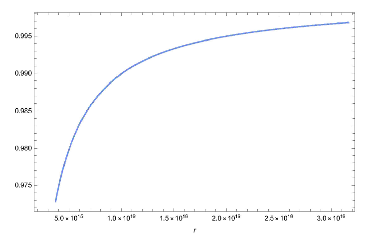
One might even obtain the region in which there would be a possible capturing of the flow, by use of an effective potential. To proceed with this method, let us use the time-like condition in Eq. (43), exploiting the total energy definition E=g00 ṫ and also Eq. (45). Rearrangement yields:

ṙ2=E2-Veff(r)2, (51)

where:

Veff(r)=(r2+1)(β(3βγ-2)-kr3+γr2-3βγr+r)r3. (52)

This potential has been plotted in Fig. 3. However, in order to capture a time-like flow, it is pretty useful to take care about the potential maximums. Such maximums may represent unstable circular orbits. Hence, if the energy of a particle is supposed to be the same as the potential maximum, it will be inevitably captured and the corresponding time-like geodesics will ultimately terminated where the potential originates from. The potential in Eq. (52) has a maximum around r≈3×1016m, where the derivatives of Veff(r) vanish. So, for this maximum and higher energies, one can expect geodesic focusing.

FIGURE 3 The effective potential for a test particle moving on a radial-directional time-like geodesic in a Weyl field. Plotting has been done for γ=10-26 m-1, β= 10-14 m and k = 10-43 m-2. 

4. Summary

In this paper, we dealt with the characteristics of time-like geodesic flows in a Weyl field and we supposed that such field is formed in vacuum spacetime obtained from vacuum Weyl field equations. We distinctly considered radial and rotational flows, and obtained their corresponding expansion, shear and vorticity (i.e. the rotation tensor). We noted that for radial flows, only expansion and shear do contribute in the characterization and as it is obvious in Fig. 1, the expansion is isotropic, however, the shear makes the formation of the curve bundle an-isotropic. Moreover, for the particular rotational flows considered here, we found that although it is not usual, however, the expansion vanishes. Therefore, we are left with a simple shear tensor and, of course, a non-vanishing vorticity. This may provide us a circular flow, which is gradually getting compact. For further considerations, one may concern with null-like geodesics in Weyl fields. Also, it is possible to take both rotation and radial motions in same flows. In cosmological contexts, this may help us to discover how real cosmic flows will behave in Weyl conformal gravity.