Research
On the anisotropic advection-diffusion equation with time dependent coefficients
H. Hernandez-Coronadoa
M. Coronadob
D. Del- Castillo-Negretec
aDepartamento de Física, Facultad de Ciencias, UNAM, Apartado Postal 50-542, Ciudad de México 04510, México.
bInstituto Mexicano del Petróleo, Lázaro Cárdenas 152, 07730, Ciudad de México, México.
cOak Ridge National Laboratory, Oak Ridge, Tennessee 37831-8071, USA.
Abstract
The advection-diffusion equation with time dependent velocity and anisotropic time dependent diffusion tensor is examined in regard to its non-classical transport features and to the use of a non-orthogonal coordinate system. Although this equation appears in diverse physical problems, particularly in particle transport in stochastic velocity fields and in underground porous media, a detailed analysis of its solutions is lacking. In order to study the effects of the time-dependent coefficients and the anisotropic diffusion on transport, we solve analytically the equation for an initial Dirac delta pulse. We discuss the solutions to three cases: one based on power-law correlation functions where the pulse diffuses faster than the classical rate ∼t, a second case specifically designed to display slower rate of diffusion than the classical one, and a third case to describe hydrodynamic dispersion in porous media.
Keywords: Time-dependent diffusion; anisotropic media; tracer and pollutant transport
Resumen
En este trabajo se analiza la ecuación de advección-difusión en la cual se tiene la velocidad y el tensor de difusión anisotrópico dependientes del tiempo, y se examinan los efectos no-clásicos del transporte y el uso de una base vectorial no ortogonal. Esta ecuación aparece en diversas áreas de la física, particularmente en transporte de partículas en campos estocásticos de velocidad y en medios porosos subterraneos, sin embargo, hace falta un análisis más profundo de sus soluciones. A fin de examinar el efecto de los coeficientes dependientes del tiempo y de la anisotropía en la difusión hemos obtenido analíticamente la solución general del modelo para el caso de un pulso inicial tipo delta de Dirac. Aplicamos la ecuación a tres casos: uno basado en funciones de correlación que siguen leyes de potencias que da lugar a super-difusión, el cual ha sido resuelto numéricamente con anterioridad, otro que hemos construido específicamente para exhibir sub-difusión, y un tercero desarrollado para describir dispersión hidrodinámica en medios porosos.
Palabras clave: Difusión dependiente del tiempo; medios anisotrópicos; transporte de trazador y contaminantes
PACS: 05.60.Cd; 05.45.Df; 47.53.+n; 47.56.+r
1. Introduction
The transport equation for a concentration field, C, analyzed in this work is obtained from the conservation law
∂C∂t=-∇⋅q
(1)
and a Fourier-Fick’s advective-diffusive closure relation of the form
q=-D(t)⋅∇C+v(t)C,
(2)
where D(t) is a symmetric diffusion tensor, and v(t) is a velocity vector field, both functions of time (not space). The resulting transport equation is
∂C∂t=∇⋅(D(t)⋅∇C-v(t)C).
(3)
Our main interest regarding the structure of the last equation concerns the time-dependence on advection and diffusion, and the anisotropy of the diffusion tensor. This equation and diverse variants of it can be found in many applications, including particle transport in anisotropic time-dependent stochastic velocity fields, where the diffusion tensor is related to velocity correlation functions. Also, tracer or pollutant transport in underground porous formations can be captured within this last approach by associating the stochastic velocity variations to permeability changes of the porous media1,2,3,4,5,6 and D is the hydrodynamic dispersion tensor that displays larger diffusion along the velocity direction than in the transversal direction. Equation (3) can be found in many other problems too, such as : (i) transport in porous materials with mixed-pore-size7, (ii) transport in periodic porous media8, (iii) transport of contaminants carried by the wind in the atmosphere9,10,11, (iv) low- and high-temperature magnetically confined plasmas, where charged particles can displace rapidly along the magnetic lines but diffuse slowly in the perpendicular (with respect to the magnetic field) direction12,13,14, (v) gas transport in cylindrical industrial ducts15,16, (vi) transport of molecular spins in bio-tissues for nuclear magnetic resonance applications17,18,19 and (vii) Brownian particles with memory, where the diffusion tensor’s time-dependence can be related to long correlations of the randomly fluctuating forces acting on the particle20,21.
In this work we obtain an analytical solution of Eq. (3) and explore the implications of the anisotropy on the transport process by examining the natural coordinate systems involved. It is to be mentioned that some practical approaches propose the description of the so called anomalous transport via a time-dependent diffusion coefficient (as in Eq. (3)), since the resulting mean square standard deviation can increase above or below the linear time dependence (as we will show later), it is interpreted as sub- or super-diffusion. As it is well-known, non-diffusive transport also naturally arises in the context of Continuous Time random Walk models with non-Gaussian and/or non-Markovian statistics see for example22,23 and references therein. However, the present work focuses on a different source of non-diffusive behavior. In particular, we are interested in systems that despite being described by Fourier-Fick’s closure relations exhibit non-diffusive transport because of the anomalous time dependence and anisotropy in the diffusion tensor.
To formulate the anisotropic transport problem on a general setting let {fi}, i = 1, … , N, denote a normalized basis of vectors in RN (not necessarily orthogonal), and write the flux as
q=∑i=1Nqifi.
(4)
Notice that the i-th component q
i
is not necessarily equal to the projection of vector q onto the basis vector f
i
, i.e., , qi=∑j=1N(q⋅fj)gji-1 where gij=(fi⋅fj) is the Euclidean metric written in the {fi} basis. This difference corresponds to the fact that q
i
are contravariant components while q⋅fj are covariant ones. If (u1,…,uN) denotes the coordinate system corresponding to the basis {fi}, then fi⋅∇=∂/∂ui.
In this work we restrict attention to homogeneous anisotropic media, such that the diffusion tensor, D, the velocity, v=∑ivifi, and the basis {fi} are space-independent quantities. Following the stochastic transport approach2,4,24, however, we keep the time dependence in both, the diffusion tensor, D(t), and the velocity, v = v(t). Furthermore, we focus on a particular class of systems characterized by the condition that their diffusion tensor can be brought to a diagonal form (with time-dependent elements), when written in the coordinate system corresponding to the basis {fi} through a time-independent linear transformation (see Eq. (9)). When, moreover, such a transformation is an element of the SO(N) group, and thus {fi} is itself an orthonormal basis, then the previous condition implies that D(t)⋅D(t')=D(t')⋅D(t) for t≠t' (this can be verified in the particular case considered in Sec. 4, see Eq. (27)). Of course this is not the most general situation by far and the physical meaning of the particular cases considered might not be straightforward at all, but for the purposes of this work, it is general enough. In fact, as will be discussed in the following sections, the “diagonalizability” condition allows us to find exact solutions to our model. The rest of the paper is organized as follows: in Sec. 2 we make some physical assumptions on the flux to define the model and we find its general solution analytically, Sec. 3 is devoted to clarify the physical interpretation of the model and in Sec. 4 we show its main features through particular examples that exhibit either normal, super or sub-diffusion. Finally, conclusions and directions of possible future work are presented in Sec. 5.
2. Model
To construct the model we assume that D is diagonal in the u-coordinate system, i.e., Dij=χi(t)δij, where δij is the Kronecker delta, and thus
qi=-χi(fi⋅∇)C+viC.
(5)
Substituting Eq. (5) into Eq. (1), and using ∇⋅fi=0, we get the transport equation
∂C∂t=∑i(χi(fi⋅∇)2C-vi(fi⋅∇)C),
(6)
or equivalently,
∂C∂t=∑iχi∂2C∂ui2-vi∂C∂ui.
(7)
Note that in the {fi} basis the transport equation in (7) is diagonal, i.e., it has no cross terms in the directional derivatives fi⋅∇. However, as we will discuss in Sec. 3 this does not necessarily imply that {fi} are the principal directions (eigenvectors) of D.
Clearly, if a different coordinate system is adopted, cross terms (involving the directional derivatives along the corresponding coordinate directions) will in general appear. As a particular important example, consider a Cartesian coordinate system (x1,…,xN) with orthonormal basis vectors e
i, i = 1, … , N. In this case,
fi⋅∇=∑jaij∂∂xj,
(8)
where the constants
aij=fi⋅ej,
(9)
define the change of bases with the corresponding change of coordinates given by the linear transformation
xi=∑jajiuj.
(10)
With inverse
ui=∑j(aT)ij-1xj=∑jAijxj.
(11)
Notice that the metric tensor can be written as gij=∑kaikajk=(a⋅aT)ij.
In the coordinates (x1,…xN) and under the assumptions made, Eq. (3) becomes
∂C∂t=∑j,kDjk∂2C∂xj∂xk-∑jvj∂C∂xj,
(12)
where vj=∑iaijvi and the diffusion tensor, Djk, is defined as
Djk=∑iχiaijaik.
(13)
Note that, by construction, Djk is symmetric, Djk=Dkj.
When written in the (u1,…uN) coordinates, the solution of the transport problem given by Eq. (7) can be obtained analytically even when χi and vi are time dependent functions. Notice that an advective-diffusive equation with time-dependent mean drift velocity, like Eq. (7), can always be written as a purely diffusive equation in terms of the rigid-translated coordinates
ui'=ui-∫0tvisds, t'=t.
(14)
If the ansatz C(u',t')=∏i=1Nhi(u'i,t') is then assumed, Eq. (7) is equivalent to the set of N equations:
∂hi∂t'=χi(t')∂2hi∂u'i2,
(15)
with i = 1, … , N, in the sense that any solution of (15) is also a solution of (7). Along this work there will be sum over repeated indices only when explicitly stated by the summation symbol. Furthermore, by introducing the temporal variables
τi(t')=∫0t'χi(s)ds,
(16)
(15) reduces to
∂hi∂τi=∂2hi∂u'i2,
(17)
for each i = 1, … , N. In order for τi to be a genuine temporal variable, it has to be a monotonic function of t, which is guaranteed since χi(t) is a positive definite function. For the initial condition hi(ui',τi=0)=δ(ui'), the solution of (17) is given by
hi(u'i,τi)=14πτiexp-u'i24τi,
(18)
and the solution of Eq. (12) is
C(x,t)=∏iexp-∑jAijxj-∫0tvi(s)ds24τi(t)4πgτi(t),
(19)
where g=detgij and Eq. (11) was used. The components of the drift velocity vector can analogously be written in the Cartesian frame according to vi=∑jAijvj.
To calculate the mean standard deviation of a pulse with respect to the normalized distribution C(u
i
, t) we define the expectation value ⟨F⟩ of a scalar function F as
⟨F⟩=∫C(ui',t')F(u')g dNu' ,
(20)
where the translated coordinate system in Eq. (14) has been used. By noticing that ⟨u'i⟩=0, it follows that
⟨ui⟩=∫0tvi(s)ds ,
(21)
which means, d⟨ui⟩/dt=vi, i.e., the mean pulse position in the f
i
direction drifts at the speed v
i
. The mean square deviation in the f
i
direction, σi2, is given by
σi2=⟨ui-⟨ui⟩2⟩=⟨u'i2⟩=2∫0tχi(s)ds .
(22)
Provided the diffusion tensor components, χi(t), Eq. (22) gives the corresponding anisotropic diffusion which, depending on χi, can be normal or anomalous.
3. Interpretation
When the f
i
basis is orthonormal (i.e., Cartesian), q
i
and fi⋅q are equal, and Eq. (5) implies that the flux along the f
i
direction depends only on the gradient of C along that same direction. However, when {fi} is not orthogonal, it can be the case that even if q
i
depends only on the gradient of C along direction f
i
, the projection fi⋅q does depend on the gradient of C along the j-th direction, for j≠i.
By choosing q
i
to obey the relation (5) and therefore the D’s components (in the {fi} basis) to satisfy Dij=χiδij, one might be tempted to conclude that the vectors of the basis {fi} are eigenvectors of the diffusion tensor. As it will be shown in what follows, it is not the case in general. In vector notation, a general eigenvalue problem can be written as
D⋅di=λidi,
(23)
where d
i
and λi are the i-th eigenvector and the corresponding eigenvalue of the second order tensor D, respectively. In particular, the dispersion tensor can be written in terms of dyadic products of the non-orthogonal basis vectors {fi}, as D=∑i,jDijfifj, where
Dij=∑k,lgik-1glj-1(fk⋅D⋅fl),
(24)
and we remind the reader that gjk-1=(fj⋅fk)-1 is the inverse of gjk=fj⋅fk, which in general is different to the identity. The existence of (fj⋅fk)-1 is guaranteed by the fact that {fi}, i=1,2,…,N, is a basis.
From expression (24) it is clear that if {fi} were eigenvectors of D, then the dispersion tensor components would be given by Dij=λigij-1. Therefore we conclude that the flux model in (5) does not imply that {fi} are the eigenvectors of
D. Moreover, since the tensor D is symmetric, its eigenvectors have to be orthogonal, and therefore they cannot be in general equal to {fi}.
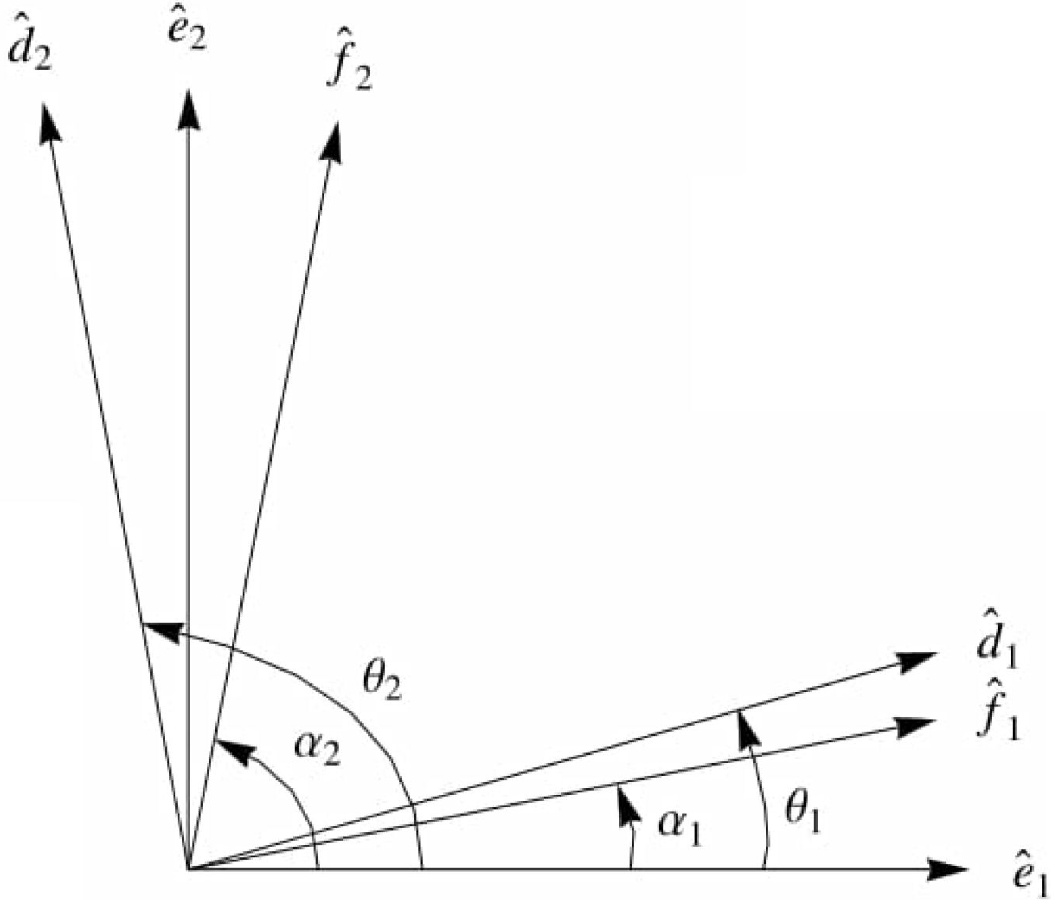
Summarizing, in general there are three different basis (see Fig. 1): (i) the non orthonormal constant basis in terms of which the problem takes its simplest form, {fi}; (ii) the Cartesian time-independent basis where the standard form of transport equation holds and our physical intuition works better, {ei}; and (iii) the time-dependent Cartesian basis defined by D’s eigenvectors, {di} (assuming they are not degenerate), which diagonalizes the diffusion tensor. It is interesting to notice that in the proposed model the coordinate system where the equation takes its simplest form is not {di}, but an auxiliary basis that allows us to solve the problem. Notice that Standard diagonalization methods are not directly applicable in this case because the diffusion tensor depends on time, its principal directions (or eigenvectors) - and therefore the associated coordinates - depend on time as well. Consequently, when written in this non-inertial coordinate system, the advection-diffusion equation contains a space and time-dependent advective term which renders it more complicated than the original one. Although these three bases are different in general, {fi} and {di} are related. This will become clear in the next examples, where we restrict attention to the case N = 2 for the sake of simplicity.
4. Applications
Let us first consider a general two-dimensional anisotropic situation. We consider a non-orthogonal basis spanned by the vectors fi=∑jaijej, with i = 1, 2, as shown in Fig. 1, with
aij=cosα1sinα1cosα2sinα2.
(25)
In such a basis, we propose a diffusion tensor whose components are written as Dij=χi(t)δij. In this case, the metric tensor in the u coordinates is:
gij= 1cos(α1-α2)cos(α1-α2) 1.
(26)
According to (13) the diffusion tensor written in Cartesian coordinates takes the form:
Dij=χ1cos2α1+χ2cos2α2χ1cosα1sinα1+χ2cosα2sinα2χ1cosα1sinα1+χ2cosα2sinα2χ1sin2α1+χ2sin2α2
(27)
and its eigenvalues and eigenvectors are:
λi=12(χ1+χ2+(-1)i+1χ12+χ22+2χ1χ2cos2(α1-α2)),di=1ni(χ1cos2α1+χ2cos2α2+(-1)i+1χ12+χ22+2χ1χ2cos2(α1-α2)χ1sin2α1+χ2sin2α2),
(29)
respectively, where n
i
is a normalization factor. Consistent with the general discussion in Sec. 3, the eigenvectors d
i
are orthonormal and different from
f
i. The vector d
1 corresponds to the direction of maximum diffusion (since λ1≥λ2). For general functions χi(t) there is not much more that can be said about d
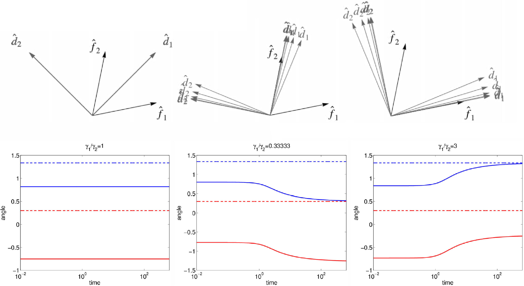
1. However, for the situation described below in cases 4.1 and 4.2, it can be shown that for large values of time t≫T (for a given characteristic decay time T) limt→∞d1=f2 for κ=χ1/χ2<1, limt→∞d1=f1 for κ>1, and d1∝f1+f2 for κ=1, shown in Fig. (2).
4.1. Anisotropic Sub-Diffusion
As a first example let us consider a case in which sub-diffusion takes place. To this end we provide an adequate form of χi(t) in the diffusion tensor. We have designed this function with the help of Eq. (22), such that σi2 exhibits the desired sub-diffusive behavior at short and long times. The resulting, at-first-glance complicated expression, is
χi(tD)=D0ie-tDtDγi-12I12-γitD,
(30)
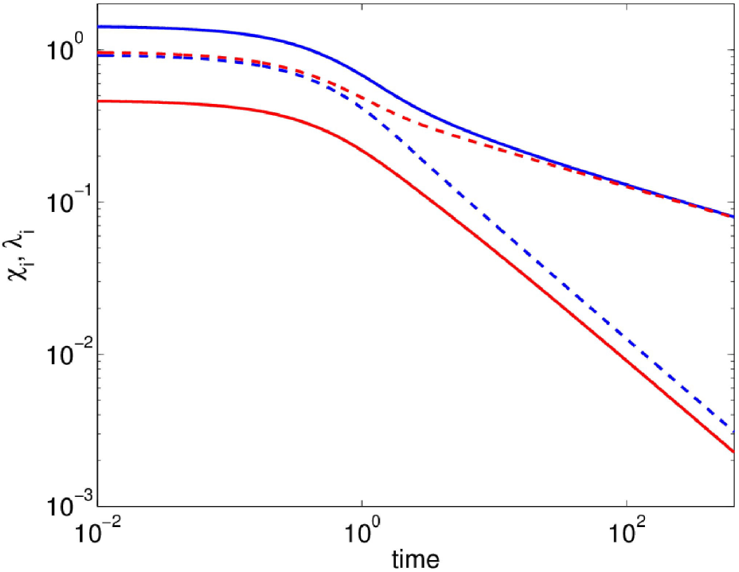
where tD=t/T, γi∈(0,1), Iα(x) is the modified Bessel function of order α and T is the system’s characteristic decay correlation time. The behavior in time of χi is relatively simple, as displayed in Fig. 3 for some values of γ. Asymptotically, it is observed that χi(t)∼tDγi-1 for tD≫1.
The corresponding mean square displacement is,
σi2D0iT=1γie-tDtDγi-1/2×((tD+1-2γi)I12-γi(tD)+tDI32-γi(tD))-2γi+1/2Γ(1/2-γi),
(31)
for γi≠1/2. For the special case of γi=1/2, the mean square displacement takes the simpler form
σi2D0iT=2e-tDtD(I0(tD)+I1tD).
(32)
For short times, tD≪1, the mean square deviation increases linearly with time for all values of γi, which corresponds to normal diffusion. However, for tD≫1 it asymptotically behaves as
σi2D0iT∼1γi2π tDγi,
(33)
which corresponds to sub-diffusion since 0<γi<1, as can be observed in Fig. 4 for tD≫1 where we show the mean square displacement as a function of time for different values of γi.
From expressions (27), (28) and (29) we know that d
1 corresponds to the direction of maximum diffusion, and also that, as shown in Fig. 2, it satisfies the asymptotic κ-dependent behaviour discussed previously, namely limt→∞d1=f2 for κ<1, limt→∞d1=f1 for κ>1, and d1∝f1+f2 for κ=1, where κ=χ1/χ2. In all cases, of course, the concentration pulse sub-diffuses according to relation (33).
4.2. Anisotropic Super-Diffusion
Let us next assume that χi(t) is given by an expression typically encountered in the theory of particle transport in random stochastic velocity fields2,4, where the diffusion coefficient is the integral of the velocity correlation function over time. If a power law correlation function is considered2,3: ξi(t)=ξ0i(1+tD)βi, it then follows
χi=D0iβi+11+tDβi+1-1βi≠-1D0iln1+tDβi=-1.
(34)
In this case, the mean square displacement takes the form:
σi24D0iT={12+βi((1+tD)βi+2-1)-tDβi≠-1,-2tD-ln(1+tD)βi=-2(tD+1)ln(1+tD)βi=-1
(35)
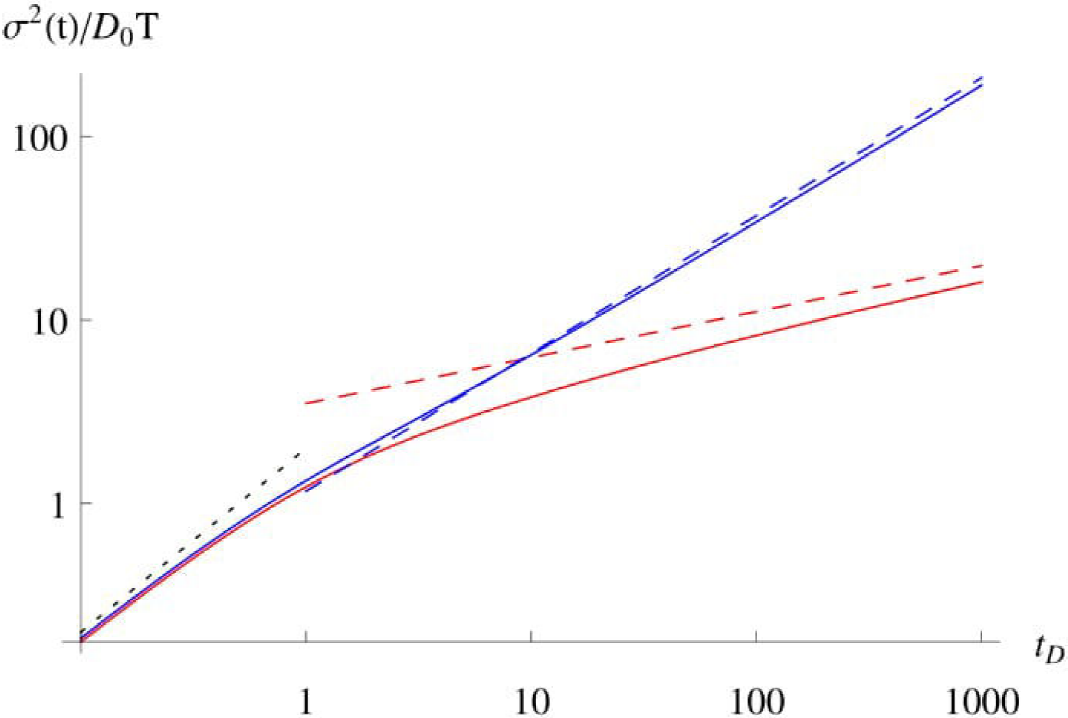
For short times, tD≪1, the mean square deviation grows as tD for βi=-1, which is diffusive; for other values of βi it increases as tD2, which corresponds to ballistic behaviour. However, for large times, tD≫1,
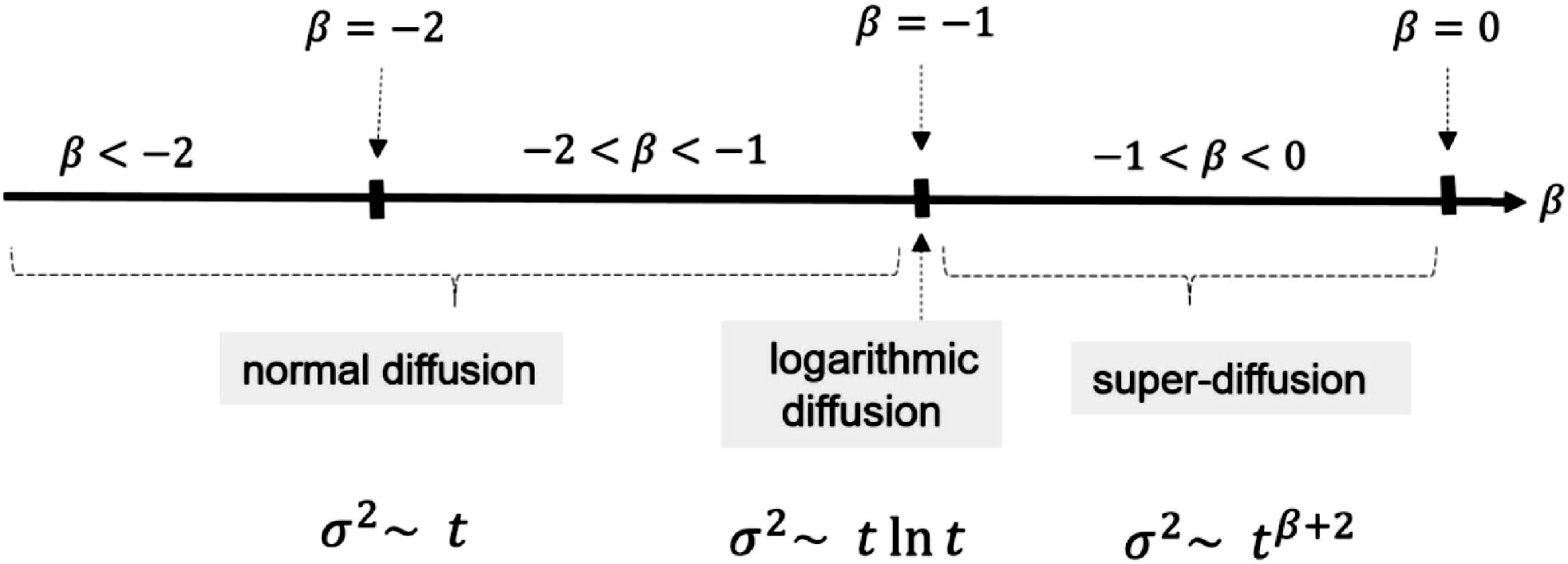
σi24D0iT∼tD|βi+1|βi<-2tDβi=-2tD|βi+1||βi+2|-2<βi<-1tDln(tD)βi=-1tDβi+2(βi+1)(βi+2)-1<βi<0
(36)
For large values of t
D
and βi=0 the diffusion is ballistic, i.e., σ2∼tD2. As shown in Fig. 5, this model describes three different asymptotic transport regimes:(i) normal diffusion for βi<-1, (ii) logarithmic-type diffusion for βi=-1 and (iii) super-diffusion for -1<βi<0.
This example has been previously studied by Numbere and Erkal3 by solving the corresponding transport equation, Eq. (12), numerically. Our analytical results confirm to certain extent their findings. In particular, for β<-3 they report “Fickian” (diffusive) behaviour in all cases. However, according to Eqs. (35) and (36), this is only true in the asymptotic regime. They describe the region -3≤β≤-1 as scale dependent or weakly diffusive, since it converges asymptotically to diffusive; this results coincides with what we analytically found, however, they logically missed (since they results are numeric) the particular case β=-1. Finally, they report the region -1≤β≤0 as “non-Fickian” (non-diffusive), which agrees with our findings. From our results, the dynamics of a pulse, as illustrated in some of their figures, can be exactly evaluated using Eq. (19).
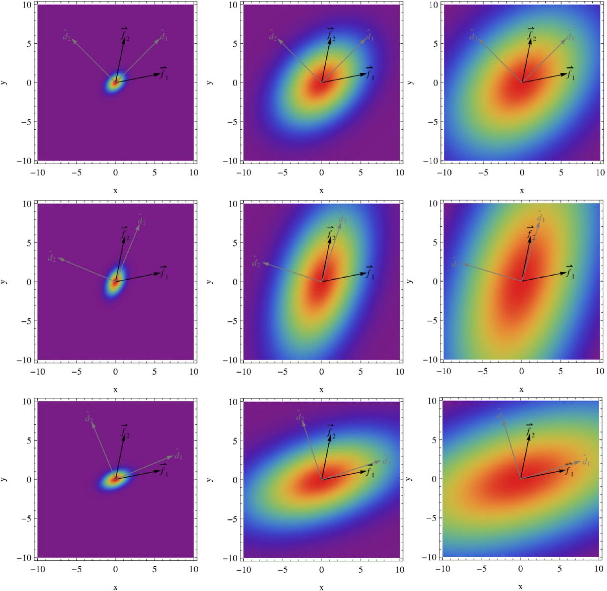
The explicit form of the concentration pulse C(x, y, t) can be found directly through expression (19). In Fig. (6) we show the time evolution of the concentration profile for three sets of parameter values (β1,β2). It can be noted that the concentration mainly diffuses along the direction d
1 which depends on the ratio κ, as we claimed: for κ<1 it tends to the direction f
2, while for κ>1 it tends to in the direction f1, when κ=1, the concentration orients along f
1 + f
2.
4.3. Hydrodynamic Dispersion
Let us finally analyse the case of hydrodynamic dispersion in an homogeneous isotropic porous media, where anisotropic dispersion appears intrinsically. The anisotropy exhibits a maximum in the velocity direction and the minimum in the perpendicular directions. In this case, the dispersion tensor is written as25,26
D=αT|v|I+(αL-αT)vv|v|
(37)
where αL and αT are the longitudinal and transverse dispersivity respectively. Since anisotropy axes are orthogonal, we choose an orthonormal vector basis with f
1 in the direction of the velocity (direction of maximum dispersion). Thus v=vf1, and therefore in a 2-dimensional system we write
Dij=vαL00αT,
(38)
and Eq. (5) gives
q1=-αLv∂C∂u1+vCq2=-αTv∂C∂u2
(40)
Thus the model of the previous subsections can be applied with χ1=αLv and χ2=αTv. Here the transformation matrix a
ij
is a rigid rotation of angle Ω from the Cartesian reference system {ei} to the {fi} system. Therefore
aij=cosΩsinΩ-sinΩcosΩ.
(41)
and Aij=(aijT)-1=aij.
Non-diffusive transport can be introduced in this model by assuming that αL=αL(t) and αT=αT(t) are functions of t conveniently chosen as it was done in the previous examples. The solution for the tracer concentration C(x1,x2,t) will be that in Eq. (19) where the proper corresponding variables are to be introduced ( Aij=aij,g=1,v2=0). In this example it is easy to see that d
i = f
i.
5. Summary and Conclusions
In this paper we have analytically solved an N-dimensional advection-diffusion equation with time-dependent coefficients and diffusion anisotropy. The problem has been formulated in terms of a non-orthogonal basis in order to accommodate anisotropy. There appear naturally two basis vector: the non-orthonormal constant basis in terms of which the problem takes its simplest form, {fi}, and the time-dependent Cartesian one defined by D’s eigenvectors, {di}, which diagonalizes the diffusion tensor. It has been shown that the coordinate system where the equation takes its simplest form is not {di} but {fi}. Although these basis are different in general, the direction of maximum dispersion, {di}, at large times, asymptotically approaches to, f
1, f
2 or f
1 + f
2, depending on the value of the ratio κ=χ1/χ2
We have particularly discussed the advection-diffusion equation in the context of its application to particle or solute transport in stochastic velocity fields. Here the diffusion tensor is given in terms of a time integral of the correlation function. The resulting transport behavior can display features of the so called sub- or super-diffusion, where the standard deviation increase in time with a power lower or lager the the unity, respectively. A known case that consider power law anisotropic dispersion coefficients2,3,24,25 was examined, and we analytically reproduced the numerical results they obtained3.
Finally, an interesting direction of future work might be to extend this model to the domain of fractional diffusion, where non-locality (in space and time) naturally arises.
Acknowledgments
This work has been partially supported by Conacyt-Sener-Hidrocarburos Fund through the project No. 143935. DdCN acknowledges support from the U.S. Department of Energy at Oak Ridge National Laboratory, managed by UT-Battalle, LLC, for the U.S. Department of Energy under contract DE-AC05-00OR22725.
References
1. G. Dagan, Flow and transport in porous formations, Springer-Verlag Berlin Heidelberg, (1989).
[ Links ]
2. Q. Zhang, Journal of Statistical Physics 66 (1992) 485-501.
[ Links ]
3. D.T. Numbere and A. Erkal, A model for tracer ow in heterogeneous porous media. SPE, (1998) pp. 37-44.
[ Links ]
4. M. Shvidler and K. Karasaki, Transport in Porous Media 50 (2003) 223-241.
[ Links ]
5. E. Morales-Casique, Sh.P. Neuman, and A. Guadagnini, Computational analysis. Advances in Water Re- sources, 29 1399-1418 (2006).
[ Links ]
6. F.A. Dorini and M.C.C. Cunha, Mathematics and Computers in Simulation (MATCOM), 82 (2011) 679-690.
[ Links ]
7. Z. Zhang, D.L. Johnson, and L.M. Schwartz, Phys. Rev. E 84 (2011) 031129.
[ Links ]
8. O.K. Dudko, A.M. Berezhkovskii, and G.H. Weiss, The Journal of Physical Chemistry B, 109 (2005) 21296-21299. PMID: 16853761.
[ Links ]
9. C.P. Costa, T. Tirabassi, M.T. Vilhena, and D.M. Moreira, Journal of Engineering Mathematics 74 (2011) 159-173.
[ Links ]
10. T. Tirabassi, M.T. Vilhena, D. Buske, and G.A. Degrazia, Journal of Environmental Protection 4 (2013) 16-23.
[ Links ]
11. M.K. Singh and N. Mahato, and N.K. Kumar, Acta Geo- physica 63 (2015) 214-231.
[ Links ]
12. P. Helander and D.J. Sigmar, Cambridge Monographs on Plasma Physics (Cambridge University Press, 2005).
[ Links ]
13. R. Balescu, Transport Processes in Plasmas. (North-Holland, 1988).
[ Links ]
14. C. Hidalgo, Astrophysics and Space Science 292 (2004) 681-69.
[ Links ]
15. Y. Mehmani and M.T. Balhoff International Journal of Heat and Mass Transfer, 78 (2014) 1155-1165.
[ Links ]
16. E. Ponsoda, E. Defez, M.D. Rosello, and J. V. Romero, Computers and Mathematics with Applications, 56 (2008) 754-768.
[ Links ]
17. L.L. Latour, P.P. Mitra, R.L. Kleinberg, and C.H. Sotak, Journal of Magnetic Resonance, Series A, 101 (1993) 342-346.
[ Links ]
18. L.L. Latour, K. Svoboda, P.P. Mitra, and C.H. Sotak, Proceedings of the National Academy of Sciences, 91 (1994) 1229-1233.
[ Links ]
19. P.N. Sen, Concepts in Magnetic Resonance Part A 23A (2004) 1-21.
[ Links ]
20. K.G. Wang and C.W. Lung, Physics Letters A 151 (1990) 119-121.
[ Links ]
21. K.G. Wang, Phys. Rev. A 45 (1992) 833-837.
[ Links ]
22. B. Berkowitz and H. Scher, Water Resources Research, 31 (1995) 1461-1466.
[ Links ]
23. B. Berkowitz, A. Cortis, M. Dentz, and H. Scher, Reviews of Geophysics, 44 (2006) 1-49.
[ Links ]
24. Q. Zhang, Advances in Water Resources, 20 (1997) 317-333.
[ Links ]
25. J. Bear, Dynamics of Fluids in Porous Media Dover Civil and Mechanical Engineering Series. (Dover, 1988).
[ Links ]
26. R.J. Charbeneau, Groundwater Hydraulics and Pollutant Transport. (Prentice Hall, 2000).
[ Links ]


 text new page (beta)
 English (pdf)
 Article in xml format
 Article references
 Send this article by e-mail
 Cited by SciELO
  Similars in
SciELO
Similars in
SciELO 
 Permalink