Introduction

The effect of wages on inflation has been a foremost subject of interest in economics. According with the traditional theory, the cost-push or the mark-up price function explain how wages increases are transferred into prices. It seems worth researching and testing this tenet empirically. In this regard, during the 1950-1960’s substantial studies were made by ^{Phillips (1958)}, ^{Dicks-Mireaux and Dow (1959)}, ^{Klein, Ball, Hazlewood and Vandome (1961)}, and ^{Lipsey and Steuer (1961)}. Continuation over similar research lines are presented in ^{Stigler (1966)}, ^{Rotemberg (1987)}, ^{Merton and Upton (1988)}, ^{Hall and Taylor (1989)}, ^{Ball and Mankiw (1995)}, ^{Romer (1996)}, ^{Pujol and Griffiths (1997)}, ^{Varian (1999)}, ^{Galí and Gertler (1999)}, ^{Woodford (2003)}, ^{Christiano et al., (2005)}, ^{Uhlig (2005)}, ^{Galí et al., (2007)}, ^{Galí (2008)}, ^{Coibion and Gorodnichenko (2013)}, ^{Mankiw (2015)}, ^{Féve and Sahuc (2017)}, and ^{Cantore et al., (2021)}.

This paper contributes to the analysis of the effect of wages on inflation in Mexican manufacturing. A mark-up price function econometric test is performed to gauge this effect. Besides, a two-period comparison, i.e., 1994-2003 and 2007-2016 is performed. An error correction econometric model is used with monthly frequency. The first period starts with the enactment of the North America Free Trade Agreement (NAFTA). A second period is associated with the beginning of the Great Recession. The econometric results could provide useful inference about the inflationary nature of wages in the Mexican case¹.

Manufacturing wage performance is gauged using an error correction model for the above-mentioned sets of periods. A first equation deals with wages and bilateral nominal exchange rate impacts on producer inflation. A second equation measures producer price index, bilateral nominal exchange rate, and wage effect on consumer inflation. These equations follow the work of ^{Pujol and Griffiths (1997)}, who use an error correction model and Granger causality tests to estimate the econometric relationships embedded in the mark-up price function. The Granger causality tests results are an informed guided to equation specification.

The error correction model results could prove or discard theoretical tenets, in this case, regarding the empiric effect of wages on inflation. The implementation of this kind of model is suitable, when there is a lack of specific data generating models in the body of traditional theory².

In this paper, wages are represented by the nominal average production wages per person for the whole manufacturing sector. The manufacturing production price index without oil represents a weighted measure of intermediary inputs costs³. The consumer price index gauges the finished goods price change. The bilateral nominal exchange rate between Mexico and the United States represents an adjustment price in an open economy, with imperfect competition and asymmetric information⁴.

Questions represented by income policies, rational expectations, the Phillips curve identification, quantitative equation, structural changes, Penn effect and their testing are beyond the scope of this research. These problems have been dealt with extensively in the literature. Evidence of these issues can be found in ^{Chow, 1960}; ^{Lucas, 1972}; ^{Wallis, 1979}; ^{Desai, 1975}; ^{Henry and Ormerod, 1978}; ^{Samuelson, 1994}; ^{Lucas, 1996}; ^{Melnick and Strohsal (2017)}, for instance.

This paper is organized as follows. Section I presents a brief literature review, where theoretical models place wages as an inflationary source. The second section presents a non-parametric data assessment by means of descriptive statistics. Besides, a figure comparison is presented for both periods under analysis, i.e., 1994-2003 and 2007-2016. Section III proposes an econometric model based on an error correction model. The econometric model is applied for Mexican manufacturing, for these two periods. Section IV examines the econometric results. Finally, the conclusions recount the empirical findings and their statistical inference.

I. Brief literature review

The inflationary nature of wages is often examined through the standard costs-push price formation model. Modifications of this basic model results on different models, i.e., the mark-up price function and inflation wage-price spirals. On one hand, the short and long term costs-push and mark-up price functions imply that, in presence of money neutrality, production costs increases are transferred fully into output prices (^{Rotemberg, 1987}). On the other hand, short term wage-price spiral function assumes price rigidities, where production costs increase is sluggishly transferred into output prices⁵.

As a modification of the costs-push model, the mark-up price function formalizes the relationship among wages, producer, and consumer prices. In the New Keynesian framework, a costs-push model is represented by a one-time shock in marginal costs. These costs could be measured through labor costs, the mark-up, or both. According with ^{Coibion and Gorodnichenko (2013)}, New Keynesian models suggest that marginal costs are a relevant source of inflationary pressures. In the New Keynesian Phillips curve labor income share is used as a proxy for marginal costs, where it could affect real quantities like the Gross Domestic Product (^{Woodford (2003)}, ^{Galí and Gertler (1999)}). ^{Galí (2008)} assumes perfect labor mobility, while capital is fixed and normalized to one.

The aggregate economic activity is examined by New Keynesians using micro foundations. In the case of ^{Christiano et al. (2005)}, wage contracts have a key role in nominal price rigidities. These rigidities could account for inertial responses in inflation, and a persistent response in output. For instance, ^{Romer (1996)} considers a short-term mark-up price function composed by sticky wages and flexible output prices. Under imperfect competition and asymmetric information his mark-up function is represented as follows:

where W stands for wages, F´(L) is the first order condition of the production function with respect to labor, WF´(L) stands for marginal costs, μ is a mark-up and P is output price⁶.

Continuing with ^{Romer (1996)}, the dynamics to establish a long-term mark-up price function considers wages at time t, as determined by prices with one period-lag t-1. In this way, price flexibility is introduced in the previous short term static equation (1). The long-term dynamic mark-up price function becomes:

where A>0 stands for a positive constant with one period-lag t-1, Pt-1 is output price with one period-lag, Wt is nominal wages at time t.

To evince the dynamics on equation (2) consider an inflationary trigger at t=1. This trigger could be either an expansionary monetary or fiscal policy. Consider that the inflationary trigger rebounds in a price increase, i.e., P1>P0, with t=1 and t-1=0.

The above inflationary trigger implies for equations (2)’ and (2)’’ that W2>W1. An inflationary wage-price spiral is already expressed in equation (2)’ and (2)’’, since Wt+1>Wt. Also, an inflationary wage price-spiral arises if A1>A0. In this case, wages are larger than those in the previous period, e.g., W2>W1. The same could happen if P1>P0. Consider now the ratio of equation (2)’’ to equation (2)’:

In general equation (3) can be expressed as Wt+1Wt=AtPtAt-1Pt-1. If the dynamics on equation (3) is maintained in each subsequent period, then wages and prices will increase each period ahead. This is because there is a mutual feedback process between equations (2)’’ and (2)’. The ratio expressed in equation (3) is expected to be positive and bigger than one, since the numerator is larger than the denominator, e.g., W2>W1. These relationships give way to a wage price-spiral where changes in magnitude are real. Now, consider that A exhibits equal values for periods 1 and 0, e.g., A1=A0.

in the expression above A1 and A0 cancels out from the last expression, assuming perfect information and absence of asymmetries. Rewritten equation (3)’ yields:

equation (3)’’ implies that changes in A are only nominal, without affecting real quantities. In equation (3)’’ money neutrality arises since nominal changes left untouched wages and prices. In this example, A plays a similar role to the well-known ^{Friedman (1956)} constant, which is often seen as a monetary policy rule. This constant could account for inflation changes in the short term (equation (3)), but neutrality in the long term (equation (3)’’). Sometimes, the Friedman constant is used to control inflation by monetary authorities⁷.

^{Pujol and Griffiths (1998)} present a variation of the previous mark-up price function, as follows:

where PPI is a manufacturing producer price index representing a proxy for output prices, WL stands for wage costs, W is wages, L is labor, PICIC is defined as the intermediate inputs costs, Y is output, μ stands for the mark-up, PICIC+WLY represents unit variable costs, PICIC+WLYα stands for marginal costs, α represents a constant share in producer prices.

^{Pujol and Griffiths (1998)} consider that output affects prices through at least two distinct channels. The first one is related with marginal costs. For example, with increasing returns to scale and holding factor prices constant, marginal costs would decline as output increases. The second channel is through the effect on the mark-up effect. According with equation (4) if the mark-up ( μ) increases, then producer prices would increase directly in the same proportion.

^{Merton and Upton (1988)} and ^{Stigler (1966)} present similar costs-push tenets. For their part, ^{Hall and Taylor (1989)} consider price formation as a positive constant time marginal cost. An analysis of the inflationary wage-price spiral is made by ^{Blanchard (1993)}. Independently, ^{Ball and Mankiw (1995)} set prices as a mark-up over marginal costs under a monopoly environment. Similar positions are held by ^{Varian (1999)}, as well as ^{Mankiw (2015)}.

The above literature review presents price formation models based on costs-push model modifications. On one hand, wages are an important component of production costs. The long-term dynamics of the model is expounded by two possible outcomes: an increase in production costs is transferred into output prices; or factor prices increases cancel out leaving real quantities without change. On the other hand, the mark-up is assumed to be payment for capital use, financial services, and depreciation costs. In brief, net domestic product after labor costs. Capital production input is an exogenous variable on the mark-up function. In this paper, only endogenous variables are dealt with in the econometric analysis. As a result, capital factor costs are not considered to be part of this research.

II. Data description

Figure analysis

In what follows, a figure analysis on annual growth rates is performed for the time series reported on table 1. The following figures represent annual growth rates, which are computed on an annual basis: month year-on-month year percentage change. One year of observations in both periods is lost because of the annual growth rates computation.

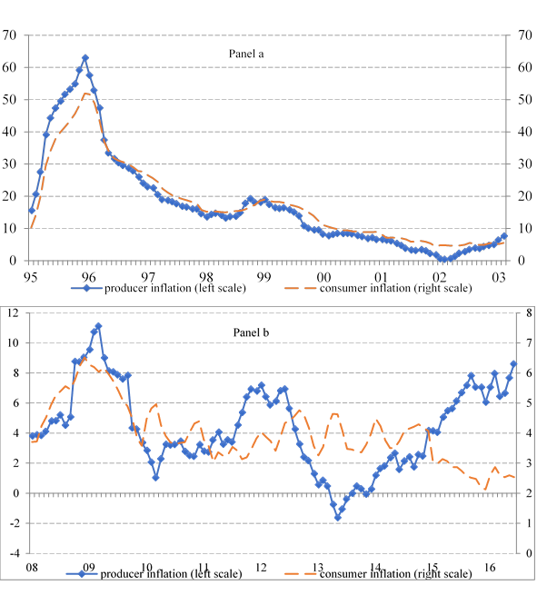
Left panels represent the period of 1995-2003, and the right panels depict the period 2008-2016. Figure 1 contains two panels depicting the same pair of variables for each period. This arrangement facilitates graphic annual growth rates comparison among periods.

Source: Own computations based on National Institute of Statistics and Geography (INEGI).

Figure 1 Mexico. Producer and consumer inflations. Annual growth rates (%). Selected periods 

Panels a and b on Figure 1 display producer and consumer inflation for the periods of 1995-2003 and 2008-2016, respectively. Panel (a) shows that producer and consumer inflation move almost hand by hand. The differences in Mean and SD for these two variables do not allow seeing this parallelism. However, their KT and CV values do because they do not have units. Therefore, they can be applied to annual growth rates description without unit problems. These statistics values are similar: 1.90 vs. 1.74 for KT, and 0.34 vs. 0.36 for CV, for each period. The high inflation depicted during 1995 could be linked with the Mexican peso devaluation of 1994. This last events account for the large axis size on panel (a). As a result, panel a registers inflation around the 60 points. Panel (b) scales do not overpass the 11 points. If, there was a lens in panel (a) around the 10 points scale, then it could be seen that there is a continuation of the producer and consumer inflation scales from period to period. The changes in scale could made the data look different across periods. Panel (b) shows almost two trends between consumer and producer inflations: simultaneity until 2009, 2011 and 2012; and only inverse for the last year.

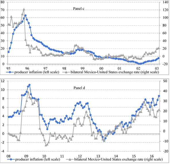
In Figure 2, Panels (c) and (d) display producer inflation and bilateral nominal exchange rate for the periods of 1995-2003 and 2008-2016, respectively. In both panels, these time series move almost in parallel way. Also, it seems that during the first and second periods there is a positive relationship between producer inflation and the bilateral exchange rate.

Source: Own computations based on National Institute of Statistics and Geography (Inegi).

Figure 2 Mexico. Producer and bilateral nominal exchange rate. Annual growth rates (%). Selected periods 

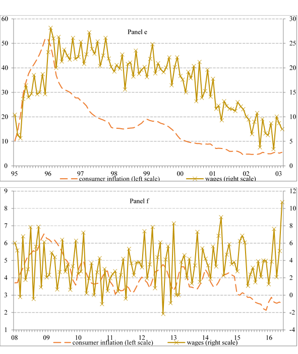
Panel (e) and (f), figure 3, show that wages have a positive relationship with respect to consumer inflation. Similar figures could be observed if wages and producer inflation were plotted¹⁰. During the period from 1995 to 2003 the growth of wages is modest with respect to consumer inflation. This behavior is reverted during the last period of 2008 to 2016, where it seems that there is less variance between wages and consumer inflation.

Source: Own computations based on National Institute of Statistics and Geography (Inegi).

Figure 3 Mexico. Producer and consumer inflations. Annual growth rates (%). Selected periods 

III. Methodology

An error correction model is applied to Mexican manufacturing. The comparison of the results is performed for two distinct periods, i.e., 1994-2003 and 2007-2016. Originally, this model was put forward by ^{Pujol and Griffiths (1998)} for the Polish economy. It has been followed by other authors, i.e. ^{Carbajal (2003)}, ^{Stockhammer et al. (2009)}, ^{Onaran et al. (2011)}, ^{Onaran and Galanis (2014)}, ^{Onaran and Obst (2015)}. In the Pujol and Griffiths model local prices are a function of labor costs and import prices. It is based on a mark-up pricing model in an imperfect competitive economy. The theoretical part of Pujol and Griffiths model has been previously exposed in section I.

^{Sargan (1964)} explains that the error correction model departs from an empirical basis. His wage-price equations are tested by means of an error correction model. This author mentions that one of the best ways to prove traditional theory is using empirical tests. This is because there is a lack of data generating models that provide unicity between theory and empirics. Other authors who test theory through this empiric lens are ^{Hickman and Klein (1984)}, ^{Hendry and Wallys (1984)}, and ^{Spanos (1995)}. In the case of ^{Cantore et al., (2021)}, they mention that in a wider set of models there is a puzzling mismatch between data and theory. Being this the present paper case, then the error correction model is suitable to prove or discard theoretical tenets.

The long-term producer and consumer price indexes reduce form follows ^{Pujol and Griffiths (1998) 11}:

where ppi represents the production price index for the whole manufacturing; w is the nominal average production wages per person for the whole manufacturing; e0 is the bilateral nominal exchange rate between Mexico and the United States; cpi stands for consumer price index; εcm5 and εcm6 stand for the error correction terms for equations (5) and (6); the subscript t stands for time ; β0, ⋯, β6 represent minimum ordinary least squares estimators.

Pujol and Griffiths explains that equation (5) measures the impact of the exchange rate on producer prices, since it affects the costs of import intermediate inputs. Also, the exchange rate may influence the mark-up of domestic firms: when the currency appreciates, margins shrink in those sectors most exposed to foreign competition.

Equation (6) is largely an account identity, as Pujol and Griffiths explain. This is in so far as it is a weighted average of producer price indices and import prices. Equation (6) incorporates wages since consumer goods are often more labor intensive than typical industrial goods. These authors mention that using exclusively the ppi would underestimate the influence of wages; besides, wages represent an important variable cost for retailers.

The numbers above each equation (5) and (6), represent the long run reduced form hypotheses. According with the New Keynesians in the long run all prices are flexible, as express in equation (3)’’. Thus, the expected values for the estimators β1, β4, β6 referring to local prices are equal to one. The bilateral exchange rate expected values β2, and β5 are also equal to one.

Equations (5) and (6) keep an analogy to the wage-price core relationships on LINK models. These models basically study national macroeconomic equilibria. In this type of models, the economic equilibria are often denoted by accounting identities (^{Hickman and Klein, 1984)}. The short-term error correction equations are:

where the symbol ∆ represents the first differences operator, and log represents the logarithmic operator. Together, these two operators allow reading the estimators as elasticities. The subscript l represents lags; (εcm5)t-1=log⁡ppit-1-β0-β1log⁡wt-1-β2log⁡e0t-1,and (εcm6)t-1=log⁡cpit-1-β3-β4log⁡wt-1-β5log⁡e0t-1-β6log⁡ppit-1. The terms ξ7 and ξ8 represent the error terms from equations (7) and (8), which are assumed to be independent and identically distributed.

The short-term equations (7) and (8) are intended to gauge the inflationary effect of wages in producer and consumer inflation. The elasticities introduce producer and consumer inflations. Thus, equations (7) and (8) test wage inflationary effects on producer and consumer inflations.

IV. Results

The results reported on table 2 indicate that for the long term, there is a positive relationship between manufacturing producer price index, wages, and bilateral exchange rate in the long and short terms. In the long term the corresponding estimators are 0.48 and 0.64 for 1994-2003, and 0.35 and 0.46 for 2007-2016. For the short-term equation (7), wage inflation effect on manufacturing producer inflation is almost nil, for both periods. That is to say, β8 is equal to 0.03 and 0.01 for each period, respectively. A similar situation is presented in equation (7), with respect to the manufacturing producer inflation and the bilateral exchange rate, where β9 is equal to 0.04 and 0.12 for each period, respectively.

The results reported on table 3 indicate that for the long term, equation (6) has a positive relationship between consumer and wage inflations: β4 has values of 0.10 and 0.07 for the periods 1994-2003 and 2007-2016, respectively. However, these estimators are close to zero. For the short-term equation (8) the wage inflation effect on consumer inflation is almost nil, for both periods. That is to say, β10 is equal to 0.01 for both periods. A similar situation is presented in the relationship between consumer inflation and the bilateral exchange rate in the short term, with β11 equal to 0.01 and 0.04, for each period respectively. In the long term, the relationship between consumer inflation and the bilateral exchange rate in equation (6) is negative, with values close to zero: -0.15 and -0.14, for each period respectively. The relationship between consumer and producer inflations in equation 8 is positive with estimators of 0.80 and 0.25, for each period respectively. Regarding this last relationship in the long term, equation (6), almost elastic transferences are registered from producer to consumer inflations are registered for both periods, i.e., 1.05 and 1.07¹².

The results reported on tables 2 and 3 do not comply with the hypothesis regarding flexible prices. Flexible prices imply that consumer and producer prices should have a unitary value at least in the long term. In contrast, the estimators reported on these tables provide insight of the presence of sticky prices in the short and long terms. In the short term the effect of wages and the bilateral exchange rate are close to nil for both periods. These results point out to a relatively weak role of wages in consumer and producer inflations. ^{Pujol and Griffiths (1998)} reach similar results in the short term where wage estimators are 0.06 and 0.20 with respect to producer and consumer inflations, respectively. According with ^{Gil Díaz and Ramos Tercero (1992)}, who examine the Mexican manufacturing sector wages are not inflationary. These authors even report negative elasticities from wages growth rate (-1.924 for 1976:09-1982:01 and -1.762 for 1982:01-1987:03), while resorting to some key inflationary prices¹³. In the case of the Euro Area, the United Kingdom, Australia, and Canada, ^{Cantore, et al., (2021)} mention that the relationship between the markup and the labor share, breaking down into a variety of models, which introduce aspects such as different production functions, fixed costs, labor market frictions, do not respond in the way models predict.

In the short term, it seems that import prices are sticky. The bilateral nominal exchange rate estimators with respect to producer and consumer inflations have values close to zero. Also, ^{Pujol and Griffiths (1998)} report inelastic coefficients (0.06) from foreign inflation to local producer inflation. ^{Gil Díaz and Ramos Tercero (1992)} mention that the exchange rate elasticity with respect to key inflationary prices was -0.921 for the 1976-1982 period in Mexico. For these authors, this result seems to indicate that the exchange rate was used to stabilize the general price level. Burtein et al. (2005) report similar results for the U.S. economy.

The bilateral nominal exchange rate is negative in the long-term equation (6) and positive in the short-term equation (8), with respect to consumer inflation. This is in so far as these estimators are close to zero. During the period 2007-2016, associated with the Great Recession, the regulation of the bilateral nominal exchange rate with two lags, contribute in the short term to a minimal increase in consumer inflation.

In the long term, the producer inflation estimators with respect to consumer inflation are 1.05 and 1.07 for each period, respectively. These values imply almost flexible prices for both periods^14,15. In the short term, the producer price inflation estimator with respect to consumer inflation are 0.80 and 0.25 for each period, respectively. Thus, producer prices are positively transferred into consumer prices, although not completely.

The long-term equation (5) and (6) do not need any lag. In the short-term equation (7) and (8) required lags: equation (7) for wages (3 lags for the period 2007-2016) and the bilateral exchange rate (1 lag for the period 1994-2013); equation (8) for wages (3 lags for the period 2007-2016) and the bilateral exchange rate (2 lags for the periods 1994-2003 and 2007-2016). Besides, equations (7) and (8) include the error correction terms with a statutory one lag¹⁶.

The results reported on table 4 indicates that the error correction terms εcm5 and εcm6 are stationary in levels, for the periods 1994-2003 and 2007-2016. The results indicate that εcm5 and εcm6 are cointegrating vectors. This result demonstrates a long-term equilibrium in equations (5) and (6), when the constant, the constant and linear trend and none tests options are considered. Thus, in the long-term equations (5) and (6) are cointegrated (^{Johansen (1988}, ¹⁹⁹², ²⁰⁰⁴⁾, and ^{Engle and Granger (1987)}). There is no need for running additional cointegration tests to prove that equations (5) and (6) are cointegrated.

The error term unit root tests indicate that εcm5 and εcm6 are stationary or integrated of degree zero. Therefore, they can be used with one lag in the short-term error correction equations. According with the results on table 4, it seems fair to argue that manufacturing producer prices, consumer prices, imported prices, and wages have common trends. This is because, these data have in common long term equilibrium information and/or share a true economic relationship (^{Sargan, 1964} and ¹⁹⁸⁴).

Regarding table 5 results, for the period 1994-2013 it cannot be rejected that wages do not Granger cause the producer and consumer price indexes, with short term probabilities of 0.0008 and 0.0010, respectively. Similar results are observed in the short term for the period 2007-2016, with respect to wages and producer and consumer price indexes: 0.0008 and 0.0010, respectively. In the short term, it cannot be rejected that the bilateral exchange rate does not Granger cause the producer price index, with probability of 0.0171 for both periods; likewise for the consumer price index: 0.0000 for both periods.

In the short term, it cannot be rejected that producer price index does not Granger cause the consumer price index, with probabilities of 0.0101 for both periods. In the long term, it cannot be rejected that the bilateral exchange rate does not Granger cause the producer and consumer price index with probabilities close to 0.0000 for both periods. In the short term, it appears that Granger causality runs one-way from wages to price indexes and not the other way. Likewise for the bilateral exchange rate and the producer and consumer price indexes; and for the producer price index and the consumer price index. In the long term, it appears that Granger causality runs one-way from the bilateral exchange rate to the producer and consumer price indexes. The pairwise Granger causality test results seems to sustain those equations (5), (6), (7), and (8) are well specified. Granger tests have not provided empirical evidence of a strong statistical causality from wage growth to inflation. Similar results have been reported by ^{Hess and Schweitzer (2000)}; ^{Hogan (1998)}; ^{Rissman (1995)}; ^{Clark (1997)} and ^{Mehra (1993)} in the United States context.

Conclusions

An error correction model in the long and short term was proposed for Mexican manufacturing, for two sets of periods: 1994-2003 and 2007-2016. Wages have an almost nil effect in manufacturing producer and consumer prices, in the long and short terms during the periods under study. The pairwise Granger causality tests have not provided empirical evidence of a strong statistical causality from wage growth to inflation tests, and signal that the error correction equations (5), (6), (7) and (8) are well specified. Together, these results are at odds with the mark-up price function traditional theoretical tenets. This body predicates upon wage increases as a source of inflation.

It appears that there are sticky import prices in the long and short terms. In the short term, the bilateral nominal exchange rate estimators respect to producer and consumer inflation are close to zero. These inflations seem unaffected by bilateral nominal exchange rate regulations. The bilateral nominal exchange rate changes from negative (equation 6) to positive (equation 8) signs, with respect to consumer inflation. This last point is a matter for further analysis.

The manufacturing producer inflation estimators, with respect to consumer prices are almost elastic in the long term. They exhibit almost unitary values in the long term for both periods. Hence, producer price index increases are almost totally transferred to consumer prices. These results suggest that there are flexible prices from the manufacturing producer to the consumer. However, in the short-term producer prices are not transferred with a unitary elasticity into consumer prices.

The long and short terms estimation results provide insight of the presence of sticky prices regarding wages. These results point out to a relatively weak role of wages in consumer and producer inflations. Thus, it seems statistically fair to infer those wages are not inflationary in Mexican manufacturing, for the periods under analysis. In this case, policies targeting wage inflation controls seem inefficient in controlling producer and consumer price inflations. As a result, policies that seek inflation control could leave wage inflation controls aside.