


 nueva página del texto (beta)
 Inglés (pdf)
 Artículo en XML
 Referencias del artículo
 Enviar artículo por email
 Citado por SciELO
  Similares en
SciELO
Similares en
SciELO 
 Permalink
1 Introduction
Motivated by the social insects’ ability to self-organize and mutually cooperate relying only on neighbor-to-neighbor communication, there has been an increasing interest during the last decade in the distributed algorithms obtaining a desired global behavior from local interactions. One of such algorithms is the consensus algorithm [15], which allows a swarm to agree on a common value in a distributed fashion (see e.g. [8,9,17,18,21,27]), using only communication among its neighbors. One of the possible applications of the consensus that achieved recently a special interest is the application to sensor networks [8]. In this scenario, of energy efficient nodes with limited computing resources, computationally simple algorithms for self-organization are of paramount importance.
It has been shown that if the underlying graph topology is strongly connected then consensus can be achieved [20]. Moreover, if the graph is balanced (identical number of in-neighbors and out-neighbors), then asymptotic convergence to the average of the swarm’s initial value is obtained by the standard consensus algorithm [20]. For graphs that are not balanced the algorithm can be modified to still achieve average consensus whenever each node has knowledge on the number of its out-neighbors [4], and compensates accordingly using a surplus variable for each node.
These results have been extended, using nonlinear theory and scalar functions used in fixed-time and finite-time stability, to achieve finite-time [11, 25, 26, 28, 30], and fixed-time convergent consensus [31, 32], (i.e. there exists a bound for the convergence time independent of the initial conditions [10, 22]). However, as we illustrate later, the convergence time does not uniquely depend on the initial conditions but mainly on the network topology, where the convergence time grows as the algebraic connectivity of the graph decreases.
In this paper, a finite-time convergence con-sensus algorithm for fixed networks is proposed. As a matter of fact, it was claimed in [28], that the consensus algorithm analyzed in the present paper could later on be justified as a consensus algorithm. Nevertheless, neither full rigorous proof, nor its sketch were provided. It is the aim of the paper to formally prove that such algorithm is a consensus algorithm for fixed networks, which is achieved using homogeneity theory [7, 14, 23]. The hereinafter proposed algorithm is shown to be computationally simpler than other finite-time consensus algorithms ( [11, 16, 28, 31]). Namely, in the proposed approach, each node requires a single computation of the nonlinear term, while in ([11,16,28,31]), the number of computations of the nonlinear term in each node equals the number of nodes adjacent to it.
Moreover, we illustrate through simulations that the proposed algorithm shows interesting robustness properties, in networks with cycle graph topology, with respect to the network growth with less control effort, namely that it shows more robustness to the network growth than previously proposed consensus algorithms. In particular, we compare our results with other consensus algorithms, namely, the asymptotic consensus [20], finite-time consensus [28] and fixed-time convergent consensus [31] algorithms.
The paper is organized as follows. In Section 2, we present the mathematical preliminaries toget-her with some previously proposed consensus algorithms. In Section 3, the main results are presented, followed by an illustrative example in Section 4. Finally, in Section 5, the conclusions and the future work are presented.
2 Preliminaries
2.1 Finite-Time Stability
We recall in this section some results on homogeneity theory [7, 14, 23] and finite-time stability [1, 2], that will be used later on. Further facts on finite time stability can be found in [2, 13, 19,24].
Definition 1. [1] Consider the nonlinear system:
Here,
where
The origin is called as finite-time convergent for(1)if there exists an open neighborhood
Note that by the uniqueness of
Definition 2. A function
if and only if:
for all
Definition 3. A vector field
Theorem 4. [2, Theorem 7.1] Let
Lemma 5. [2] The right-hand side of:
where
Lemma 6. [29,32] Consider the non-homogeneous system:
then the origin of(4)is finite-time stable and uniformly convergent (i.e. the bound on the convergence time is independent of the initial conditions) and its settling-time is bounded by
2.2 Graph Theory
The following notation and preliminaries on graph theory are taken mainly from [12].
A graph
For the Laplacian
A path from
2.3 Asymptotic, Finite-Time and Fixed-Time Convergent Consensus
In this subsection we present the standard consensus algorithm with asymptotic convergence and describe how nonlinear algorithms are derived from it, with particular focus on finite-time and fixed-time convergent algorithms.
Let
where
where
Considering nonlinear functions
and on the other hand with the algorithm:
There by, the consensus algorithms proposed in [28] and [32] are derived from (3) and (4), respectively, following the direction (7). Namely, the finite-time consensus algorithm proposed in [28] is:
The fixed-time convergent algorithm proposed in [31] for fixed topologies is:
where
Although, both [28] and [32] ([28] does not present the proof of the claim), address the consensus derived from (3) and (4), respectively, following also the direction (8), the results in both papers are restricted to static networks, i.e. where
3 Main Results
In this section we derive the mathematical proofs to show the finite-time convergence to the consensus state of the proposed algorithm under fixed networks. First, we show using Lyapunov theory, the asymptotic convergence to the consensus state. Then, the finite-time convergence follows by using homogeneity [5-7,14,23] and Theorem 4.
The aim of this paper is to show that, if
where
Remark 7. Notice that using the proposed consensus algorithm (11), a node requires a single computation of the nonlinear function
Remark 8. In [28] it was shown that(9), is a consensus algorithm with finite-time convergence. The authors claimed (without proof), that using their framework, it can be shown that for ”static networks”(11), is also a consensus algorithm with finite-time convergence. In the following we provide a rigorous proof, using Lyapunov theory and homogeneity theory [14,23], to show that(11), is a consensus algorithm with finite-time convergence in fixed communication networks.
Let
where
Thus, the dynamic for
where
In the following, (13) will be referred as the error dynamics. The
Lemma 9. Let
In the case when
Proof. Straightforward.
Proposition 10. Let
is globally asymptotically stable.
Proof. Consider the candidate Lyapunov function
Then according to Subsection 2.2, there exists a factorization for the graph Laplacian
where the equality in (15), for the case when
However, since
Lemma 11. Let
Proof. Notice that the function
Now, let the
Since
The main result of this paper is the following.
Theorem 12. Let
Proof. According to Proposition 10, the dynamic of
Remark 13. Notice that the convergence time for the case when
4 An Illustrative Example Showing Robustness to the Network Growth
In this section we illustrate that, in networks with cycle graph topology, the convergence of the proposed consensus algorithm (11), is more robust to the network growth than the standard consensus algorithm (6) proposed in [20], the finite-time consensus algorithm (9) proposed in [28] and the fixed-time convergent algorithm (10) proposed in [31] while requiring less control effort. To this end, we consider a communication topology described by an undirected cycle graph
We simulate three different scenarios to illus-trate the convergence of the above mentioned consensus algorithms with respect to the network growth (the simulation was performed using the Modelica® language and simulated in Dymola® using the Euler integration method). Namely, a network formed by an undirected cycle graph
We would like to highlight that the initial conditions are set the same for the different algorithms using the linear congruential generator [3]:
where
Table 1 Parameters selected for the different algorithms
| Algorithm | Parameters |
|---|---|
| Proposed Algorithm |
|
| Asymptotic Consensus (6) |
|
| Finite-time Consensus (9) |
|
| Fixed-time Consensus (10) |
|
The evolution of the above mentioned algorithms for a cycle graph
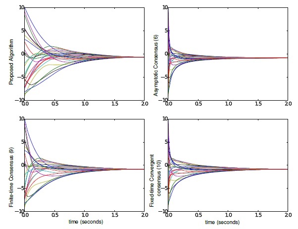
Fig. 1 Different consensus algorithms experimentally set for convergence to the consensus state approximately at 2 seconds under a cycle graph
Now, let us consider the control effort related to each agent as
Table 2 Total energy comparison among the different algorithms
| Algorithm | Total Energy |
|---|---|
| Proposed Algorithm | 26.44 |
| Asymptotic Consensus (6) | 83.00 |
| Finite-time Consensus (9) | 37.49 |
| Fixed-time Consensus (10) | 64.21 |
However, as the number of agents under a cycle graph communication topology grows (i.e. as the smallest nonzero eigenvalue decreases), the convergence time to the consensus state varies among the different algorithms.
For instance, when it grows from 25 to 200 agents the convergence of the asymptotic consensus algorithm grows from 2 seconds to approximately 120 seconds, as shown in Fig. 2. The consensus of the finite-time consensus of [28] grows to 20 seconds, the fixed-time convergent one to 30 seconds whereas the proposed consensus algorithm grows from 2 seconds to 7 seconds.
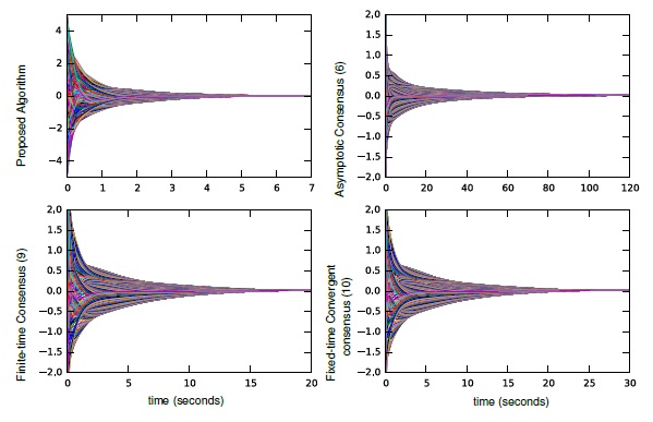
Fig. 2 Comparison among different consensus algorithms when the network grows to 200 agents with communication topology
Moreover, as the cycle network grows to
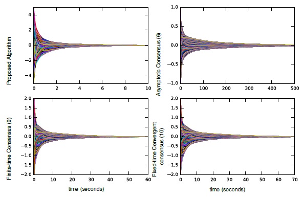
Fig. 3 Comparison among different consensus algorithms when the network grows to 1000 agents with communication topology
It is worth noting that in many scenarios the network size is not determined a priori and in general it cannot be estimated by the agent to adjust accordingly.
Thus, algorithms that could be used over a wide range of scenarios (different network size and topology) with a single parameter configuration are desirable, contrary to algorithms whose convergence-time varies so widely that it becomes prohibited (as the asymptotic consensus algorithm of Fig. 2) in some applications.
5 Conclusions and Future Work
A continuous-time consensus algorithm with finite-time convergence over fixed networks was presented in this paper. Finite-time convergence was proven using homogeneity theory.
The proposed algorithm is computationally simpler than previously proposed finite-time con-sensus algorithms. Moreover, the proposed approach was compared, in simulations with existing consensus algorithms, including the standard consensus algorithm and finite-time and fixed-time convergent algorithms, showing its robustness, in a cycle graph topology, to the network growth.
Future work concerns the analysis of the proposed algorithm under dynamic networks which will be reported elsewhere.

