


 nueva página del texto (beta)
 Inglés (pdf)
 Artículo en XML
 Referencias del artículo
 Enviar artículo por email
 Citado por SciELO
  Similares en
SciELO
Similares en
SciELO 
 Permalink
1. Introduction
The spatial and temporal variations of the Earth’s magnetic field (EMF), recorded in various geological and archaeological materials such as volcanic rocks, ceramics and sediments, facilitate the reconstruction of the secular behavior of the EMF over extended time periods. Globally, an increasing body of paleomagnetic and archaeomagnetic studies has contributed a substantial amount of directional and intensity data concerning the EMF from Holocene volcanic events and human occupation sites over the past 5,000 years. These data have enabled the development of global models that describe the paleosecular variation (PSV) of the EMF in different regions of the world. Models such as SHA.DIF.14K (Pavón- Carrasco et al., 2014), CALS10k.2 (Constable et al., 2016) and ArchKalmag14k (Schanner et al., 2022), among others, offer insights into the secular variations of the EMF, with the precision of these models contingent upon the availability, quality and accuracy of regional data across specific time periods. Hence, the necessity for expanding the temporal and spatial scope of available data remains paramount.
Such models enable the construction of synthetic secular variation curves, which, among other applications, allow for the dating of volcanic and archaeological materials up to approximately 14,000 ka, by using specialized techniques (e.g., Pavón-Carrasco et al., 2011). The accuracy achieved with these methods is comparable to that obtained through radiometric dating techniques, such as radiocarbon dating (C14).
In Mexico, several regional secular variation curves have been developed (e.g., Goguitchaichvili et al., 2018b; Mahgoub et al., 2019; Hervé et al., 2019, García-Ruiz et al., 2021) based on paleomagnetic data from volcanic and archaeological materials originating from Mexico and Central America. Most of the data from volcanics and archeological materials, used for regional curves in Mexico and global models, are available on different databases such as LAPOD (Rodríguez-Trejo et al., 2024). These models have been employed to date volcanic events and archaeological contexts, with their reliability and precision corroborated by numerous studies conducted across a variety of settings and time periods (e.g., Böhnel et al., 2016; Alva-Valdivia et al., 2021; Rodríguez-Trejo et al., 2023). Nonetheless, further data on the EMF’s direction and intensity are required to enhance the quality and resolution of existing regional and global models. This expansion of the data set will allow for improved dating accuracy and a deeper understanding of the spatial and temporal behavior of the EMF.
This study presents archaeointensity results and magnetic properties’ analysis of ceramic fragments from four archaeological sites located in the Yucatán Peninsula, Mexico (Figure 1), which correspond to the Maya civilization during distinct phases of Mesoamerican occupation (Figure 2). The Maya civilization was one of the most prominent and developed societies in Mesoamerica, occupying a vast area that extended over southern Mexico, Guatemala, El Salvador and Honduras. It had an almost continuous presence from approximately 2000 B.C.E. to the colonial period. In the region, different geophysical studies have been conducted with the aim of achieving a non-invasive survey of the different archaeological zones, including Chichén-Itzá (e.g., Tejero-Andrade et al., 2019; Cárdenas-Soto et al., 2024). Archaeomagnetic studies have also been carried out in the region and generally in the Maya area, where data from archaeological materials such as kilns, ceramics and burnt soils, among others, have been obtained (e.g., Alva-Valdivia et al., 2021; Goguitchaitchvili et al., 2018a, 2020; Ortiz-Ruiz et al., 2024).
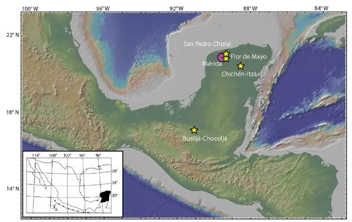
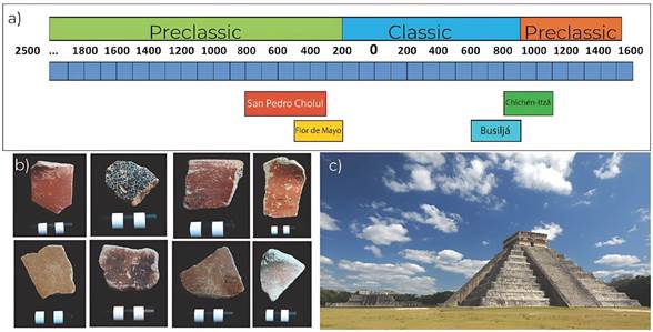
Figure 2. a) Chronological framework of the pottery sherds and archaeological sites, spanning from 2500 B.C.E. to 1600 A.D.; b) Representative pottery sherds analyzed in this study; c) The Temple of Kukulcán, Chichén-Itzá (image modified from www.inah.gob.mx).
The chronology used for the sites in this study spans portions of the Preclassic (2500 B.C.E.-200 A.D.), Classic (200 A.D.-900 A.D.) and Postclassic (900 A.D.-1521 A.D.) periods, based on archaeological context and stratigraphy. In addition, four archaeomagnetic dating were conducted to accurately determine the age of each period. Ceramics and their associated chronological relationships were provided by archaeologists from the Universidad Autónoma de Yucatán, drawing on research projects carried out at the sites of Chichén-Itzá, Flor de Mayo, San Pedro Cholul and Busiljá-Chocoljá. The dating of these materials was established through an analysis of each site’s archaeological context, including known occupation periods, stratigraphy and the typological sequence of the recovered fragments. Each ceramic piece was retrieved from the same stratigraphic level as its corresponding dated context, thereby ensuring temporal consistency. Additionally, the samples correspond to six different ceramic types: Dzitas Pizarra (e.g., Cobos 2001), Chinikiha (e.g., Obando et al., 2011), Sierra rojo (e.g., Balcárcel et al., 2010), Xanaba rojo (e.g., Gallareta et al., 2012), Juventud Rojo (e.g., Quiñones-Cetina, 2006), and Chunhinta negro (e.g., Rissolo et al., 2005), which are associated with four distinct periods: Terminal Late Classic (700-1100 A.D.), Late Classic (600-900 A.D.), Late Preclassic (300 B.C.E.-250 A.D.), and Middle Preclassic (800-300 B.C.E.). Table 1 shows the age period associated with each sample; general chronology is displayed in Figure 2.
Table 1 Summary of reported archaeointensity results, including their associated ceramic type and the age period estimated by typology.
| Specimen | Period | Ceramic type | Site |
|---|---|---|---|
| MAYAS02 | Terminal Late Classic 700-1100 A.D. | Dzitas Pizarra | Chichén-Itzá |
| MAYAS06 | Terminal Late Classic 700-1100 A.D. | Dzitas Pizarra | Chichén-Itzá |
| MAYAS08 | Terminal Late Classic 700-1100 A.D. | Dzitas Pizarra | Chichén-Itzá |
| MAYAS09 | Late Classic 600-900 A.D. | Chinikiha | Busljá-Chocoljá |
| MAYAS10 | Late Classic 600-900 A.D. | Chinikiha | Busljá-Chocoljá |
| MAYAS05 | Late Preclassic 300 B.C.E.-250 A.D. | Sierra rojo | Flor de Mayo |
| MAYAS14 | Late Preclassic 300 B.C.E.-250 A.D. | Xanaba rojo | Flor de Mayo |
| MAYAS11 | Middle Preclassic 800-300 B.C.E. | Joventud Rojo | San Pedro Cholul |
| MAYAS16 | Middle Preclassic 800-300 B.C.E. | Chunhinta negro | San Pedro Cholul |
2. Methodology
This study encompasses 24 ceramic sherds from four different archaeological sites (Figure 1). Each sherd was divided into 6 to 8 small fragments for the archaeointensity protocol (Figure 3a and 3b). Magnetic properties of the samples were measured at the Paleomagnetism Laboratory of the Institute of Geophysics, UNAM. A small fragment from each ceramic piece was selected for magnetic susceptibility as a function of temperature (k-T) measurements, utilizing an MFK2 susceptibility-meter (Agico, Kappabridge). The fragments were ground into powder and heated from room temperature to a maximum of 20 °C. The heating and cooling processes were conducted in an Argon atmosphere to minimize oxidation effects during thermal treatment. For the magnetic hysteresis and isothermal remanent magnetization (IRM) experiments, a fragment of approximately 25 mg from each ceramic piece was sectioned. The measurements were conducted using a Princeton 2900 MicroMag Alternating Gradient Magnetometer (AGM), applying a maximum magnetic field of 1.2 Tesla.
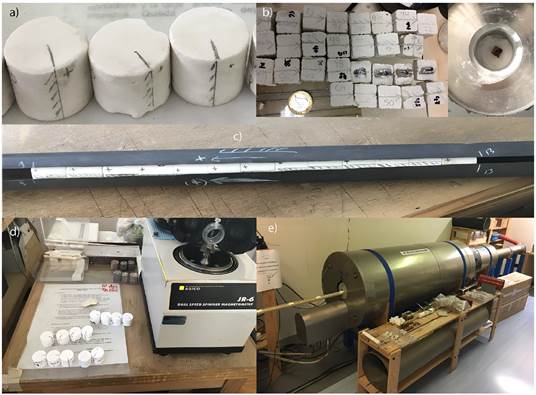
Figure 3. a) Sample assembly in salt cylinders (2.5 cm in diameter); b) Mounting of samples in a high-temperature-resistant diamagnetic plaster matrix; c) Sample holder used for heating samples embedded in salt; d) JR-6 spin magnetometer at IGF-UNAM; e) 2G cryogenic magnetometer at CEREGE-CNRS.
To determine archaeointensity, the samples were processed at both the Rock Paleomagnetism Laboratory of the Institute of Geophysics, UNAM and the Paleomagnetism Laboratory of CEREGE-CNRS & Aix-Marseille University, France. The double-heating protocol proposed by Thellier and Thellier (1959) was employed, wherein each sample is subjected to two thermal cycles while a laboratory magnetic field is applied along the +Z and -Z axes. During the experiments, partial thermo-remanent magnetization (pTRM) checks (Coe, 1967) were performed after every two temperature steps to verify potential magnetic mineralogical alterations during heating. The samples were heated in magnetically shielded rooms at both UNAM (67% of the samples) and CEREGE-CNRS (33% of the samples), with temperature increments ranging from 200 °C to 580 °C, while applying a magnetic field of 40 µT. The remanent magnetization was measured using an AGICO JR-6 spinner magnetometer at UNAM and a 2G Enterprises cryogenic magnetometer at CEREGE-CNRS. Data processing and interpretation were performed using the web-based application paleointensity.org (Beguin et al., 2020) and the software ThellierTool 4.22 (Leonhardt et al., 2004).
Given the nature of general ceramic manufacturing, anisotropic thermoremanent magnetization (ATRM) may occur, potentially introducing biases in archaeointensity estimates (Rogers et al., 1979; Aitken et al., 1988), often leading to overestimations or underestimations of intensity values. To mitigate this effect, it is essential to correct for anisotropy by calculating the ATRM tensor (Veitch et al., 1984; Chauvin et al., 2000). This correction involves four additional heating steps as part of the Thellier-Thellier procedure, using the final temperature of the heating process. Successive measurements are performed along six sample orientations corresponding to the +x, −x, +y, −y, +z, and −z axes. The last two measurements include the final heating step of the Thellier-Thellier process, followed by a thermal alteration check.
The anisotropy correction was applied individually to each specimen, with a correction factor for ATRM estimated for each sample, following the methodologies outlined by Veitch (1984) and Chauvin et al. (2000).
3. Results
3.1. MAGNETIC PROPERTIES
3.1.1 MAGNETIC SUSCEPTIBILITY AS A FUNCTION OF TEMPERATURE (K-T)
The curves obtained from the k-T experiments were classified into two groups according to their reversible behavior and similar Curie temperature (Tc), as shown in Figure 4. The first group, which represents 25% of the specimens, shows two magnetic phases: the first between 320 °C and 370 °C (Figure 4a) and another between 450 °C and 520 °C. The second group, corresponding to 75% of the specimens, also exhibits two or more magnetic phases, the first between 150 °C and 180 °C (Figures 4b, 4c and 4d), and another between 400 °C and 450 °C. In both groups, the predominant magnetic carrier is associated with a transition between Ti-rich and Ti-poor titanomagnetites.
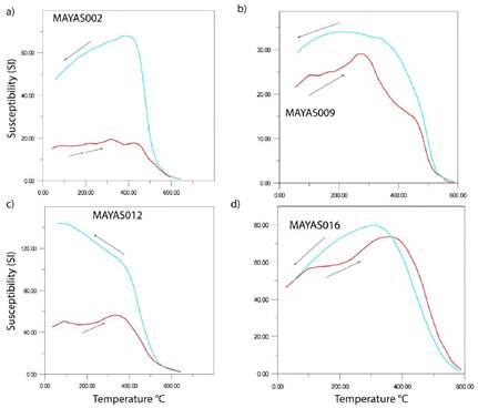
Figure 4. Summary of representative susceptibility vs. temperature experiments. The red curve represents the heating process, while the blue curve corresponds to the cooling process.
In 90% of the results, a low level of reversibility is observed, where cooling curves show susceptibility values that increase by up to 300% compared to the heating curve. This indicates significant mineralogical alteration during the heating process, with the formation of new magnetic minerals such as magnetite and other titanomagnetites with varying Ti content. The specimen with the greatest reversibility corresponds to the one shown in Figure 4d. In 25% of the cases, a small magnetic phase near 620 °C is detected, which could correspond to titanohematite, possibly a product of alteration and oxidation during burial, along with exposure to moisture and pedogenic processes.
3.1.2. MAGNETIC HYSTERESIS
The results of the magnetic hysteresis experiments reveal a diverse mixture of magnetic minerals. All measurements were normalized by specimen mass. In 80% of the samples, a characteristic potbellied behavior (Figures 5b, 5c and 5d) was observed, indicating predominantly pseudo-single domain (PSD) behavior, as described by Tauxe et al. (1996, 2002).
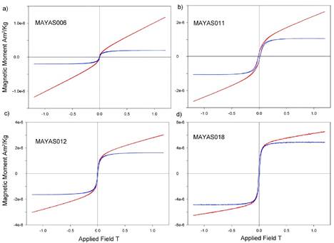
Figure 5. Summary of representative curves of magnetic hysteresis experiments. The curve in red shows the result of the mass normalized experiment. The blue curve shows the mass normalized results after correction for the contribution of paramagnetic mineralogy.
In the remaining specimens, a wasp-waisted behavior was identified, suggesting a mixture of minerals with both low and high coercivity, such as titanomagnetite and titanohematite (Figure 5a). Saturation magnetization values range from 150 mT to 300 mT, coercivity values between 4.2 mT and 9.6 mT and squareness ratio values between 0.104 and 0.26 (Mrs/Ms). These values indicate a trend from small to medium-sized magnetic grains typical of PSD structures (Tauxe et al., 2002), transitioning towards larger grains associated with multi-domain (MD) structures. This transition is evident in the Day plot (Day et al., 1977), where a shift from PSD to MD particles is observed (Figure 6). Data from the Chichén-Itzá, San Pedro Cholul and Flor de Mayo sites show good clustering, while the Busiljá-Chocoljá site, located further from the Chichén-Itzá region, exhibits more variability.
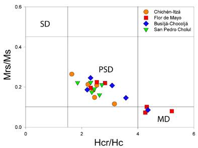
Figure 6. Day plot shows the results of magnetic properties (domain state) for each sherd, represented by an archaeological site.
Both the k-T and hysteresis curves confirm a consistent identification of the dominant magnetic mineralogy. The results indicate that the magnetic carriers are primarily titanomagnetite and magnetite, with lesser contributions from high- coercivity minerals such as titanohematite. The predominance of titanomagnetite and magnetite is evidenced in the k-T curves and further supported by the potbellied hysteresis loops. Similarly, the presence of titanohematite is corroborated by both the k-T curves and the wasp-waisted behavior observed in the hysteresis loops.
3.2. ARCHAEOINTENSITY
The preparation of ceramic pieces followed two different methodologies. In the paleomagnetism laboratory at UNAM, 16 out of 24 ceramic pieces were processed. Each piece was cut into six cubic fragments (5 mm per side), which were embedded in a diamagnetic matrix of powdered salt. The fragments were then compacted under pressure into 2.5 cm diameter cylinders (Figures 3a, 3c and 3d). In the paleomagnetism laboratory at CEREGE-CRNS, 8 out of 24 ceramic pieces were processed, cutting six fragments from each piece, shaped as parallelepipeds of 5x3x15 mm, and embedded in a matrix of a high-temperature- resistant diamagnetic gypsum compound (Figures 3b and 3e).
Archaeointensity experiments were conducted on 144 specimens obtained from 24 ceramic fragments across four archaeological sites (Figure 1). To ensure the reliability of the results, eleven quality criteria were established based on the parameters proposed by Paterson et al. (2014) and the acceptance standards described for the ThellierTool software (Leonhardt et al., 2004).
The number of heating steps (n) used to calculate the best-fit linear segment in the Arai- Nagata diagram (Nagata et al., 1965) must be at least 5. The standard error ratio (β) should remain below 0.15, while the fraction (f), representing the proportion of total thermoremanent magnetization (TRM) included in the linear fit, must exceed 35%. Additionally, the gap factor (g), which evaluates the uniformity of temperature intervals, needs to be greater than 0.5 and the quality factor (q), reflecting the overall reliability of the fit, must be higher than 3.
The maximum angular deviation (MAD), as defined by Kirschvink (1980), should not surpass 10°. Furthermore, δCK, which is the maximum absolute difference generated by partial TRM (pTRM) checks and normalized by the total TRM, is required to be less than 9%. The cumulative alteration parameter, δpal, determined by the difference between corrected and uncorrected intensity estimates, must be under 18%. The parameter |k’|, representing the inverse of the radius of the best-fit circle to the Arai plot data, should not exceed 0.27.
For each ceramic fragment, at least three specimens must yield valid results to calculate a reliable archaeointensity mean and the standard deviation (σ) of these values must not exceed 5 μT. Based on the aforementioned criteria, reliable archaeointensity values were obtained for 30 out of 144 processed specimens (Table 2), representing up to 21% of the total samples. The remaining results were excluded from the final analysis for failing to meet the minimum parameters required to be considered valid for paleointensity estimates. In some cases (up to 25%), the results were discarded due to the presence of a strong secondary magnetization component (Figure 7d), likely caused by reheating or alteration processes. Additionally, approximately 50% of the samples were rejected because they did not meet all the established criteria for reliable archaeointensity determination. In all these cases, the specimens were disqualified from further analysis.
Table 2 Summary of archaeointensity results. B lab : Laboratory-applied field; Espec: Specimen; N: Number of points used to estimate the slope in the Arai-Nagata plots; f: Fraction of NRM; g: Gap factor; q: Quality factor; MAD: Maximum angle of deviation; β: Standard error ratio; Banc: Estimated archaeointensity in microtesla (µT); Bσ: Archaeointensity standard deviation; F ATRM : Estimated correction factor for ATRM; BATRM: Archaeointensity corrected by the ATRM value; B CDMX : Archaeointensity relocated to a reference location in central Mexico; VADM: Virtual axial dipole moment estimated in ZAm².
| Site | Spacimens | n | f | s | q | β | MADanc | α | δCk | δpal | |k'| | B anc | Bσ | FATRM | BATRM | BCDMX | VADM | Class | Mean B | Estimated age |
|---|---|---|---|---|---|---|---|---|---|---|---|---|---|---|---|---|---|---|---|---|
| Chichén-Itzá | MAYAS02A | 5 | 0.44 | 0.7 | 15 | 0.02 | 4 | 11.95 | 6.2 | 14.5 | 0.01 | 37.3 | 2 | 1.12 | 41.8 | 41 | 9.18 | B | 39.8 ± 2.5 | 800-1100 A.D. |
| Chichén-Itzá | MAYAS02D | 6 | 0.48 | 0.74 | 16 | 0.022 | 3.4 | 9.52 | 6.3 | 9.6 | 0.04 | 35 | 1.1 | 0.981 | 34.3 | 33.7 | 7.54 | A | ||
| Chichén-Itzá | MAYAS02E | 7 | 0.57 | 0.79 | 20 | 0.023 | 3.1 | 5.65 | 6.1 | 8.6 | 0.03 | 38.8 | 1.3 | 0.998 | 38.7 | 38 | 8.51 | A | ||
| Chichén-Itzá | MAYAS02F | 8 | 0.61 | 0.81 | 11 | 0.044 | 3 | 10.07 | 6.6 | 9.6 | 0.25 | 42 | 2.2 | 1.06 | 44.5 | 43.7 | 9.78 | A | ||
| Mean by sherd | 38.3 | 2.9 | 39.8 | 39.4 | 8.83 | |||||||||||||||
| Chichén-Itzá | MAYAS06C | 6 | 0.55 | 0.79 | 5 | 0.086 | 3.5 | 5.54 | 8.6 | 15.5 | 0.24 | 37.7 | 4.1 | 1.05 | 39.6 | 38.8 | 8.7 | B | ||
| Chichén-Itzá | MAYAS06D | 7 | 0.69 | 0.82 | 10 | 0.06 | 4.1 | 2.46 | 7.3 | 17.5 | 0.045 | 37.4 | 4.5 | 0.995 | 37.2 | 36.5 | 8.18 | B | ||
| Chichén-Itzá | MAYAS06E | 8 | 0.76 | 0.85 | 9 | 0.069 | 3.5 | 4.32 | 8.7 | 16.6 | 0.14 | 40.7 | 3.1 | 0.998 | 40.2 | 39.4 | 8.83 | B | ||
| Chichén-Itzá | MAYAS06F | 9 | 0.99 | 0.85 | 11 | 0.08 | 3.8 | 2.11 | 7.8 | 17.6 | 0.21 | 42.7 | 3.2 | 0.998 | 42.4 | 41.6 | 9.32 | B | ||
| Mean by sherd | 40.6 | 4.3 | 39.8 | 39.1 | 8.75 | |||||||||||||||
| Chichén-Itzá | MAYAS08B | 7 | 0.62 | 0.75 | 6 | 0.075 | 7.5 | 9.84 | 8.9 | 11.9 | 0.008 | 44.9 | 3.1 | 0.905 | 39.8 | 39.1 | 8.75 | B | ||
| Chichén-Itzá | MAYAS08E | 8 | 0.69 | 0.79 | 10 | 0.057 | 6.9 | 10.24 | 7.8 | 14.7 | 0.12 | 47 | 3.5 | 0.943 | 44.3 | 43.5 | 9.74 | B | ||
| Chichén-Itzá | MAYAS08F | 9 | 0.84 | 0.83 | 10 | 0.073 | 6.3 | 8.46 | 6.3 | 16 | 0.26 | 41.8 | 4.2 | 1.008 | 42.1 | 41.3 | 9.26 | B | ||
| Mean by sherd | 44.6 | 2.6 | 42.4 | 41.5 | 9.31 | |||||||||||||||
| Busiljá | MAYAS09A | 4 | 0.5 | 0.51 | 5 | 0.049 | 5 | 9.83 | 5.2 | 16.9 | 0.134 | 34.2 | 1.2 | 1.091 | 37.3 | 38.3 | 8.58 | B | 37.7 ± 2.5 | 600-900 A.D. |
| Busiljá | MAYAS09D | 5 | 0.55 | 0.58 | 6 | 0.049 | 4.3 | 6.59 | 5.3 | 12.5 | 0.212 | 35.3 | 0.9 | 1.098 | 38.8 | 39.9 | 8.95 | A | ||
| Busiljá | MAYAS09G | 6 | 0.55 | 0.57 | 4 | 0.074 | 4.2 | 7.22 | 6.4 | 14.8 | 0.047 | 33.9 | 2.2 | 1.09 | 36.95 | 38.1 | 8.54 | B | ||
| Mean by sherd | 34.5 | 1.7 | 37.7 | 38.8 | 8.69 | |||||||||||||||
| Busiljá | MAYAS10C | 7 | 0.61 | 0.63 | 5 | 0.077 | 4.4 | 8.36 | 8.7 | 16.4 | 0.223 | 32.1 | 3.2 | 0.998 | 32.04 | 32.9 | 7.37 | B | ||
| Busiljá | MAYAS10D | 8 | 0.61 | 0.63 | 5 | 0.072 | 4.2 | 14.25 | 7.7 | 17.9 | 0.208 | 37.3 | 2.8 | 0.987 | 36.8 | 37.9 | 8.45 | B | ||
| Busiljá | MAYAS10F | 9 | 0.62 | 0.63 | 6 | 0.064 | 4.2 | 12.92 | 8.8 | 17.6 | 0.268 | 38 | 2.4 | 0.997 | 37.9 | 39.1 | 8.74 | B | ||
| Mean by sherd | 35.8 | 3.2 | 35.6 | 36.6 | 8.17 | |||||||||||||||
| San Pedro Cholul | MAYAS05B | 6 | 0.51 | 0.79 | 5 | 0.075 | 9.2 | 14.63 | 6.8 | 17.2 | 0.253 | 61.1 | 4 | 0.997 | 60.9 | 59.7 | 13.38 | B | 59.7 ± 4.2 | 300 B.C.E.-250 A.D. |
| San Pedro Cholul | MAYAS05C | 7 | 0.64 | 0.83 | 10 | 0.056 | 9.6 | 13.5 | 7.7 | 17.3 | 0.054 | 58.5 | 3.7 | 0.978 | 57.2 | 56.1 | 12.57 | B | ||
| San Pedro Cholul | MAYAS05E | 9 | 0.78 | 0.87 | 10 | 0.066 | 7.8 | 14.2 | 6.4 | 12.9 | 0.243 | 53.5 | 2.7 | 0.986 | 52.8 | 51.7 | 11.59 | B | ||
| Mean by sherd | 57.7 | 3.2 | 56.8 | 56.1 | 12.01 | |||||||||||||||
| San Pedro Cholul | MAYAS14C | 6 | 0.48 | 0.8 | 7 | 0.052 | 3.3 | 5.06 | 8.9 | 9.1 | 0.201 | 72.2 | 4.7 | 0.89 | 64.3 | 63 | 14.12 | A | ||
| San Pedro Cholul | MAYAS14D | 7 | 0.64 | 0.83 | 10 | 0.052 | 2.8 | 4.12 | 7.8 | 8.9 | 0.137 | 66.9 | 2.1 | 0.915 | 61.2 | 60 | 13.45 | B | ||
| San Pedro Cholul | MAYAS14F | 8 | 0.71 | 0.85 | 15 | 0.04 | 2.9 | 4.35 | 8.7 | 8.3 | 0.043 | 67.9 | 2.5 | 0.995 | 67.6 | 66.2 | 14.84 | B | ||
| San Pedro Cholul | MAYAS14E | 9 | 0.85 | 0.87 | 20 | 0.038 | 2.4 | 3.45 | 8.1 | 9.6 | 0.142 | 65.1 | 1.8 | 0.963 | 62.7 | 61.5 | 13.77 | A | ||
| Mean by sherd | 68 | 3.1 | 63.9 | 62.7 | 14.05 | |||||||||||||||
| Flor de Mayo | MAYAS11D | 6 | 0.55 | 0.78 | 6 | 0.071 | 2 | 1.56 | 3.4 | 9.1 | 0.235 | 52.5 | 3.2 | 0.994 | 52.2 | 51.2 | 11.47 | A | 53 ± 5.3 | 800-300 B.C.E. |
| Flor de Mayo | MAYAS11E | 7 | 0.74 | 0.82 | 10 | 0.058 | 1.7 | 1.47 | 4.1 | 7.6 | 0.209 | 49.2 | 4.7 | 0.981 | 48.3 | 47.4 | 10.62 | A | ||
| Flor de Mayo | MAYAS11F | 8 | 0.79 | 0.83 | 14 | 0.047 | 2.6 | 1.67 | 3.3 | 6.5 | 0.217 | 48.1 | 4.4 | 0.998 | 48 | 47.1 | 10.55 | B | ||
| Mean by sherd | 49.9 | 2.3 | 49.5 | 48.6 | 10.9 | |||||||||||||||
| Flor de Mayo | MAYAS16A | 7 | 0.65 | 0.8 | 6 | 0.138 | 2.8 | 4.54 | 7.9 | 14.9 | 0.267 | 59.6 | 1.8 | 0.989 | 58.9 | 57.8 | 12.95 | B | ||
| Flor de Mayo | MAYAS16B | 8 | 0.69 | 0.81 | 5 | 0.105 | 3.4 | 5.9 | 8.3 | 13.9 | 0.236 | 60.8 | 2.1 | 0.995 | 60.5 | 59.3 | 13.29 | B | ||
| Flor de Mayo | MAYAS16E | 9 | 0.73 | 0.83 | 6 | 0.098 | 3.4 | 6.06 | 7.7 | 13 | 0.147 | 56.6 | 4.3 | 0.998 | 56.5 | 55.4 | 12.41 | B | ||
| Mean by sherd | 59 | 2.1 | 58.6 | 57.5 | 12.88 | |||||||||||||||
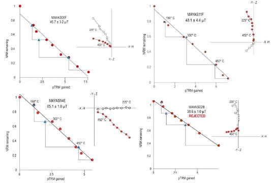
Figure 7. Summary of representative archaeointensity results. Arai-Nagata plot with stability checks (on the left) and thermal demagnetization diagram (right).
From the 30 archaeointensity measurements, 9 mean values were obtained for the four archaeological sites analyzed in this study. The intensity values ranged from 32 ± 3.2 μT to 67.6 ± 2.5 μT, while the virtual axial dipole moments (VADM) varied between 7.37 ZAm² and 14.84 ZAm² (Figure 7).
Table 2 presents the archaeointensity results that meet the established quality criteria. Each Banc value was corrected by multiplying it by its respective FATRM, yielding the intensity value corrected for anisotropy (BATRM). In most cases, the correction factor fell within the range of 1% < FATRM < 12%. This correction process refines the intensity estimates by reducing the anisotropy effect, which otherwise leads to overestimation or underestimation of the Earth’s magnetic field (EMF) intensity in the analyzed samples.
Figure 9 compares the obtained results (Table 2) with two regional PSV curves (Mahgoub et al., 2019; García-Ruiz et al., 2021) and the global model SHA.DIF.14k (Pavón-Carrasco et al., 2014). To facilitate this comparison, the BATRM results were relocated to a reference point in central Mexico at 19.43° N, 99.13° W, corresponding to Mexico City’s center. These adjusted values are presented in Table 2, under the BCDMX column.
A general agreement is observed between the archaeointensity values and the expected intensities from the PSV models, according to the estimated age of each sample. However, the archaeointensity results for the MAYAS05 specimen (Table 2) exhibit a maximum angle of deviation (MAD) between 5° and 10°, which is higher than that of the other specimens, where deviations remain below 5°. Despite this, the result meets the minimum acceptance criteria for archaeointensity studies.
3.3. ARCHAEOGMAGNETIC DATING
Archaeomagnetic dating was conducted using the MATLAB tool Archaeodating (Pavón- Carrasco et al., 2011) in combination with the global geomagnetic models SHA.DIF.14k (Pavón-Carrasco et al., 2014) and SHAWQ2k (Campuzano et al., 2019), as well as the regional intensity PSV model (García-Ruiz et al., 2021). The age estimation was performed within a chronological range spanning from 1500 B.C.E. to 1500 A.D (Figure 8).
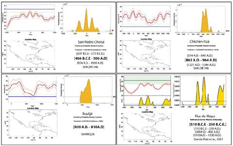
Figure 8. Archaeomagnetic dating results obtained using different PSV curves, analyzed with the Archaeodating MATLAB tool (Pavón-Carrasco et al., 2014).
For each sample, up to three age ranges were derived from the applied PSV models, in addition to the chronological constraints provided by the archaeological context associated with each ceramic type. To integrate these multiple estimates into a single representative age, a Bayesian approach was applied, incorporating the uncertainties associated with each interval. Bayesian inference is widely employed in chronological studies due to its ability to integrate prior knowledge and rigorously quantify uncertainty (Buck et al., 1996; Gelman et al., 2013).
For each given range (Ai,Bi), the central value was estimated as:
and the uncertainty was estimated:
Assuming a uniform distribution within the interval. The final estimated age was derived through a weighted combination of the different sources based on their variances:
where μpost represents the best estimate for the combined age. The posterior variance was estimated as:
That quantifies the contribution of the uncertainty from each individual estimate and improves the precision of the final result (Gelman et al., 2013). From these values, a 95% confidence interval was established using:
providing a more reliable and statistically robust age range.
This method is particularly useful in chronological analysis when integrating data from different dating techniques or sources, as it allows for a probabilistic combination of independent estimates (Buck et al., 1996). In the field of radiocarbon dating, Bayesian models have been extensively used to refine age determinations and to assess the consistency of different dating methods (Ramsey, 2009). After the Bayesian approach, 4 new ages were constrained based on the dating of the ceramic types, from the Middle Pre-Classic to the Terminal Late Classic. Table 3 summarizes the determined ages after the archaeomagnetic dating and the Bayesian inference.
Table 3 Summary of archaeomagnetic dating results based on different PSV curves, along with the estimated age using Bayesian inference.
| Site | Estimated age range | PSV curve used for dating | Archaeomagnetic dating |
|---|---|---|---|
| Chichén-Itzá | 800-1100 A.D. | Ceramic type dating | 859-975 A.D. |
| 785-1165 A.D. | García-Ruiz et al., 2021 | ||
| 426-809 A.D. | SHAWQ2K | ||
| 862-964 A.D. | SHA.DIF.14k | ||
| Busiljá-Chocoljá | 600-900 A.D. | Ceramic type dating | 689-864 A.D. |
| 795-1150 A.D. | García-Ruiz et al., 2021 | ||
| 430-810 A.D. | SHAWQ2K | ||
| 527-956 A.D. | SHA.DIF.14k | ||
| Flor de Mayo | 800-300 B.C.E. | Ceramic type dating | 623-488 B.C.E. |
| 510-250 B.C.E. | García-Ruiz et al., 2021 | ||
| 956-506 B.C.E. | SHA.DIF.14k | ||
| San Pedro Cholul | 300 B.C.E.-250 A.D. | Ceramic type dating | 31 B.C.E.-170 A.D. |
| 85 B.C.E.-190 A.D. | García-Ruiz et al., 2021 | ||
| 38 B.C.E.-364 A.D. | SHAWQ2K | ||
| 466 B.C.E.-506 A.D. | SHA.DIF.14k |
4. Discussion
The results of the magnetic properties analysis reveal consistency in terms of the thermal and magnetic stability of the samples. The k-T curves predominantly display two distinct magnetic phases, characterized by high and low Curie temperatures. Additionally, the hysteresis curves indicate minimal magnetic mineralogical mixing, with saturation magnetization values remaining below 300 mT. The magnetic domain behavior primarily follows a pseudo-single domain (PSD) trend, with a minor component exhibiting multi-domain (MD) characteristics. These findings suggest that the dominant carriers of magnetization are titanomagnetites with varying titanium content.
The ratios of magnetization (Mrs/Ms) and coercivity (Hcr/Hc), as illustrated in the Day diagram, exhibit similar patterns across the Flor de Mayo, Chichén-Itzá and San Pedro Cholul archaeological sites. However, the results from Busiljá-Chocoljá show slight deviations.
One of the main limitations of existing global and regional paleosecular variation (PSV) models is the reliability of data reported in recent years. In some cases, paleomagnetic and archaeomagnetic data, both directional and intensity, fail to meet the minimum quality standards required for them to be considered reliable, introducing a significant source of error in the resulting models. Additionally, the dating of many samples often carries a high degree of uncertainty, and in some cases, chronological corrections or refinements are made over time, further increasing the uncertainty of the available models.
To ensure the reliability of the data, archaeointensity results were selected based on previously established quality criteria. An anisotropy effect was observed, directly associated with the ceramic manufacturing process. The ATRM correction improved the accuracy and precision of the results, revealing systematic overestimations in archaeointensity, which, on average, ranged between 5% and 10%.
The relocation of BCDMX results to central Mexico enabled direct comparisons with PSV intensity curves from other regions of the country, such as those compiled by Mahgoub et al. (2019) and García-Ruiz et al. (2021), which primarily include records from central Mexico. Additionally, the results were compared with the global geomagnetic model SHA.DIF.14k (Pavón-Carrasco et al., 2014).
Despite the broad range of estimated ages, as shown in Figure 9, the obtained values remain within acceptable limits and align with the expected secular variation trends for the analyzed time period.
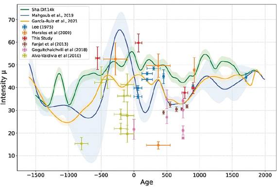
Figure 9. Comparison of archaeointensity results from this study with regional and global PSV models over the past 3,000 years.
As observed in Figure 9, the values obtained in this study for the Late Classic period are consistent with the expected values from the PSV models presented. The result obtained for the Middle Preclassic period closely aligns with both the SHA. DIF.14k model and the reconstruction proposed by Mahgoub et al. (2019). In contrast, the estimated value for the Late Preclassic period shows a slight deviation from SHA.DIF.14k and Mahgoub et al. (2019), and a more marked discrepancy when compared with the model proposed by García- Ruiz et al. (2021). These discrepancies among the PSV models can be attributed to the limited availability of intensity data for this period (on all the PSV models), which affects the robustness of the PSV curves.
Figure 9 also presents a comparison with previously published archaeointensity values from sites in the Maya region (e.g., Lee, 1975; Morales et al., 2009; Alva-Valdivia et al., 2010; Fanjat et al., 2013; Goguitchaichvili et al., 2018a), revealing a pattern of both agreements and discrepancies with current PSV models. These inconsistencies emphasize the need to expand the available archaeointensity dataset to enhance the accuracy and resolution of PSV reconstructions for Mesoamerica. Data for comparison were obtained from LAPOD (Rodríguez-Trejo et al., 2024).
5. Conclusions
The results obtained in this study provide valuable insights into the magnetic properties and archaeomagnetic dating of ceramic materials from four archaeological sites in the Maya region, which were occupied from the Middle Preclassic to the Early Postclassic period. These findings reveal similarities in the raw materials used for ceramic production, as well as in the magnetic mineralogy responsible for carrying the remanent magnetization, which enabled the archaeointensity analysis. The results confirm that the primary magnetic carriers are titanomagnetites with varying titanium content.
The Earth’s magnetic field intensity values were selected based on strict quality criteria to ensure a high level of reliability. The archaeointensity results range from 32 ± 3.2 μT to 67.6 ± 2.5 μT, while the virtual axial dipole moment (VADM) values range from 7.37 ZAm² to 14.84 ZAm². These findings are consistent with expected values according to regional and global paleosecular variation (PSV) models for the last 3,000 years in Mexico.
The comparison of the results with regional and global PSV models highlights the need for further refinement of PSV curves for southeastern Mexico and Central America, a region rich in archaeological remains and Holocene volcanic materials but with limited published studies (e.g., Alva-Valdivia et al., 2010; Rodríguez- Trejo et al., 2023). Therefore, the integration of paleomagnetic and archaeomagnetic data, including both intensity and directional records, combined with high-precision dating, is essential for the development of more robust and refined PSV models for the region.
Additionally, the archaeomagnetic dating of four ceramic types from four archaeological sites provides valuable chronological constraints for each site. These results not only contribute to refining the archaeological context but also demonstrate the reliability and applicability of the paleomagnetic method as a chronological tool for Mesoamerican archaeology.

