SciELO - Scientific Electronic Library Online

 
vol.70 número5An exact treatment of localization of electromagnetic plus separable potentialPhase signal analysis for high-sensitive temperature fiber-optic external Fabry-Perot-cavity sensor índice de autoresíndice de materiabúsqueda de artículos
Home Pagelista alfabética de revistas  

Servicios Personalizados

Revista

Articulo

Indicadores

Links relacionados

  • No hay artículos similaresSimilares en SciELO

Compartir


Revista mexicana de física

versión impresa ISSN 0035-001X

Rev. mex. fis. vol.70 no.5 México sep./oct. 2024  Epub 07-Oct-2025

https://doi.org/10.31349/revmexfis.70.051301 

Optics

Solitary wave type solutions of nonlinear improved mKdV equation by modified techniques

R. K. Alhefthia 

M. Ishfaq Khanb 

J. Sabi’uc 

D. Nawaz Khan Marwatd 

M. Ince 

a Department of Mathematics, College of Sciences, King Saud University, P.O. Box 2455, Riyadh 11451, Saudi Arabia.

b Department of Mathematics, COMSATS University Islamabad, Pakistan.

c Department of Mathematics, Yusuf Maitama Sule University, Kano, Nigeria.

d Department of Mathematics, Faculty of Technologies and Engineering Sciences, Islamia College Peshawar, 25120, Jamrud Road, University Campus, Peshawar, Khyber Pakhtunkhwa, Pakistan.

e Department of Mathematics, Firat University, 23119 Elazig, Turkiye. e-mail: minc@firat.edu.tr


ABSTRACT

In this paper, the improved and modified version of the Sardar sub-equation method (IMSSEM) and the improved generalized Riccati equation mapping method (IGREMM) are manipulated effectively and generously to determine the exact solitary wave soliton solutions of the improved modified KdV (mKdV) equation. The purpose of this study is to provide novel exact solutions to the improved mKdV equation. Specifically, we utilized IMSSEM and IGREMM to study different solutions of the nonlinear improved mKdV equation, focusing on exponential, trigonometric, and trigonometric hyperbolic type solutions. Furthermore, the plotting of various solutions for direct viewing analysis is provided in two and three-dimensional graphs. The new strategies are straightforward, quick, and efficient and have many other advantages, whereas, they provide the most accurate and unique solution to many other types of nonlinear partial differential equations (NPDEs), which usually arise in engineering and applied sciences. It should be noted that these methodologies are novel mathematical instruments that have shown to be the most effective mathematical tools for solving higher-order nonlinear partial differential equations in mathematical physics. Symbolic computation was used to validate all of the solutions that were established. Thus, it is also hoped that these techniques will ultimately reduce the cumbersome workload involved during the process of solutions to complicated NLPDEs.

Keywords: IMSSEM and IGREMM; improved mKdV equation; solitary wave solution; NLPDEs

1 Introduction

The nonlinear partial differential equations (NLPDEs) have been used extensively for the simulation of many problems of physical nature, whereas, they have exactly described and controlled the behavior of such phenomena. However, such NLPDEs are used frequently for the simulation of problems in fluid mechanics, structural engineering, optical fiber, plasma physics, biology, solid state, and physical sciences. Besides that the techniques for finding the exact solutions to NLPDEs are rare. On the other hand, few handsome strategies have been devised for the solutions of NLPDEs in recent years, however, it is a big miracle in the world of mathematics. Note that the details of such techniques can be found in the literature, e.g. Tan-cot [1, 2], sine-cosine [3, 4, 12], extended trail method [5, 6], new auxiliary equation [7, 8, 9], Jacobi elliptic ansatz [10, 11], Hirota’s direct [14, 15], extended direct algebraic [13, 16, 17], generalizes Bernoulli sub-ODE [18, 19], function variable [20, 21], sub-function [22, 23], and others [24, 25, 26, 27, 28, 29, 30, 31, 32, 33, 34, 35, 36, 37]. Strictly speaking, we categorically emphasized the effectiveness of the two important and modified techniques, i.e. IMSSEM and IGREMM and they are utilized here wisely to produce the solitary wave solutions of the nonlinear improved mKdV equation. These solitary wave solutions of the improved mKdV equation are important in the application of KdV equations in science, engineering, and physics. The improved mKdV equation is:

ut+au2ux+buxxt+βuxxx=0, (1)

where the unknown function u(x,t) is the dependent variable and it has varied with x and t. The improved mKdV equation has an extra dispersive term, i.e. the part of Eq. (1) which contains b This modification creates many significant changes in the solution structure. The improved mKdV equation is one of the perfect models useful in electromagnetic and elastic media, whereas, it explains the nonlinear wave propagation in polarity and symmetric systems. Therefore, we focused its solutions on improved and modified algorithms which are very effective and efficient, whereas, they may solve other nonlinear problems of a complex nature in a very easy way and preserve the physical characteristics of the problem.

Furthermore, the article is briefly managed: In Sec. 2, we explained the description of the proposed methodology IMSSEM and IGREMM. In Sec. 3, we applied the IMSSEM and IGREMM to construct the novel exact, most accurate solitary wave solutions of the improved mKdV equation. In Sec. 4, the 2D and 3D graphs are plotted for direct viewing study and in Sec. 5, we outlined the conclusion.

2 Methodology of the proposed improved techniques

Analyze the nonlinear PDEs

F(u,ut,ux,uxx,), (2)

where the function u = u(x,t) is an unknown function. At the moment, we introduced the following wave transformation

u=uξ,  ξ=x-ct, (3)

where c0, by using the transformation in (3) into (2) to reduce the nonlinear PDE and to convert it into a nonlinear ODE with an integral order.

Nu',u'',u''',. (4)

We have solved the above non-linear ODE by using IMSSEM and IGREMM these techniques have the following standard forms:

            uξ=a0+j=1Najϕj(ξ)  aN0, (5)

where, a j (j = 0,1,,2,3,..,N).

The value of N can be determined by balancing the highest order derivative term and the highest order nonlinear term in Eq. (5). Therefore, the highest degree of dru/dξr is classified as:

Odrudξr=n+r,    r=1,2,3,. (6)

                  Ouqdrudξr=q+1n+r,    q=0,  1,2,, (7)

and r = 1,2,3,…

2.1 The enhanced Sardar sub-equation approach

The ϕ(ξ) in Eq. (5) is considered the solution to the following equation:

ϕ'2ξ=δ2ϕ4ξ+δ1ϕ2ξ+δ0, (8)

where δi,i=0,1,2   are constants to be determined. The following set of solutions satisfies Eq. (8) where C is the integration constant:

1. For δ0=δ1=0 and δ2>0, we obtained the rational solutions:

ϕ1±(ξ)=±1δ2(ξ+C), (9)

2. For δ0=0 and δ1>0, the exponential solutions will be of the form:

ϕ2±(ξ)=4δ1e±δ1ξ+Ce±2δ1ξ+C-4δ1δ2, (10)

ϕ3±(ξ)=±4δ1e±δ1(ξ+C)1-4δ1δ2e±2δ1(ξ+C). (11)

3. The trigonometric hyperbolic solutions are as follows:

4. For δ0=0, δ1>0 and δ20, we have

ϕ4±(ξ)=±-δ1δ2sechδ1ξ+C   (12)

ϕ5±(ξ)=±δ1δ2cschδ1ξ+C  . (13)

5. For δ0=δ12/4δ2, δ1<0 and δ2>0, we have

ϕ6±(ξ)=±-δ12δ2tanh-δ12ξ+C  , (14)

ϕ7±(ξ)=±-δ12δ2coth-δ12ξ+C  , (15)

ϕ8±(ξ)=±-δ12δ2(tanh-2δ1ξ+C  ±isech-2δ1ξ+C  , (16)

ϕ9±(ξ)=±-δ12δ2(coth-2δ1ξ+C  ±csch-2δ1ξ+C  , (17)

ϕ10(ξ)=±-δ18δ2(tanh-δ18ξ+C  +coth-δ18ξ+C  . (18)

6. The solutions which have the form of trigonometric functions are presented below:

7. For δ0=0, δ1<0 and δ20, we have

ϕ11±(ξ)=±-δ1δ2sec-δ1ξ+C, (19)

ϕ12±(ξ)=±-δ1δ2csc-δ1ξ+C. (20)

8. For δ0=δ12/4δ2, δ1>0 and δ2>0, we have

ϕ13±(ξ)=±δ12δ2tanδ12ξ+C  , (21)

ϕ14±(ξ)=±δ12δ2cotδ12ξ+C  , (22)

ϕ15±(ξ)=±δ12δ2(tan2δ1ξ+C  ±sec2δ1ξ+C  , (23)

ϕ16±(ξ)=±δ12δ2(cot2δ1ξ+C  ±csc2δ1ξ+C  , (24)

ϕ17±(ξ)=±δ18δ2(tanδ18ξ+C  -cotδ18ξ+C  ), (25)

Remember that we have substituted Eqs. (5)-(8) into Eq. (4) and equated all the coefficients of each power of ϕ(ξ) to zero and solved the resultant system of algebraic equations with the help of Maple. Eventually, we incorporated these constants (coefficients) into Eq. (5) and obtained the solution of distinct types as shown in Eqs. (9)-(25). As a result, we obtained different exact solutions for NPDEs.

2.2 The enhanced generalized Riccati equation mapping method

The ϕ(ξ) in Eq. (5) is the solution of

ϕ'ξ=β2ϕ2ξ+β1ϕξ+β0, (26)

where βi,i=0,1,2   are constants and they need to be determined later. The following set of solutions is obtained with the integration constant c:

1. For β0=β1=0 and β20, the rational solutions will be of the form:

ϕ1±(ξ)=±1β2(ξ+C), (27)

2. For β0=0, the solution of the exponential type is simply obtained as:

ϕ2ξ=-β1ϕβ1(e-β1ξ+C+φ)  , (28)

ϕ3ξ=-β1eβ1ξ+Cβ2(eβ1ξ+C+φ)  , (29)

3. For ρ=β12-4β0β1>0, β1β20 or β0β20, and p and q be nonzero real constants, the solutions presented in the form of trigonometric hyperbolic functions are given below:

ϕ4ξ=-ρ2β2tanhρ2ξ+C-β12β2  , (30)

ϕ5ξ=-ρ2β2cothρ2ξ+C-β12β2  , (31)

ϕ6±ξ=-ρ2β2(tanhρξ+C  ±isechρξ+C-β12β2, (32)

ϕ7±ξ=-ρ2β2(cothρξ+C±cschρξ+C  )-β12β2, (33)

ϕ8ξ=-ρ4β2(tanhρ4ξ+C  +coth  ρ4ξ+C-β12β2, (34)

ϕ9±(ξ)=±ρ(p2+q2)-pρcosh(ρξ+C)2β2p  sinhρξ+C+q  -β12β2, (35)

ϕ10(ξ)=2β0cosh  ρ2ξ+C  ρ  sinhρ2ξ+C-β1coshρ2ξ+C, (36)

ϕ11ξ=2β0sinh  ρ2ξ+C  ρcoshρ2ξ+C  -β1sinhρ2ξ+C  , (37)

ϕ12±ξ=2β0cosh  ρξ+C  ρsinhρξ+C  -β1coshρξ+C  ±iρ, (38)

ϕ13±ξ=2β0sinh  ρξ+C  ρcoshρ(ξ+C)-β1sinhρξ+C  ±ρ, (39)

ϕ14ξ=2β0sinhρ4ξ+C  coshρ4ξ+C2ρcosh2ρ4ξ+C-2β1sinhρ4ρξ+C  coshρ4ξ+C  -ρ  . (40)

4. For ρ=β12-4β0β2<0,  β1β20 or β0β20, the solutions of the trigonometric form are demonstrated as follows:

ϕ15ξ=-ρ2β2tan-ρ2ξ+C-β12β2  , (41)

ϕ16ξ=--ρ2β2cot-ρ2ξ+C-β12β2  , (42)

          ϕ17±ξ=-ρ2β2  tan-ρξ+C  ±sec-ρξ+C-β12β2  , (43)

ϕ18±ξ=--ρ2β2cot-ρξ+C  ±csc-ρξ+C  -β12β2, (44)

ϕ19(ξ)=-ρ4β2tan-ρ2ξ+C-cot-ρ4ξ+C  -β12β2, (45)

ϕ20±ξ=±-ρ(p2-q2)-p-ρcos-ρξ+C  2β2psin(-ρξ+C+q-β12β2, (46)

    ϕ21ξ=-2β0cos-ρ2ξ+C  -ρsin-ρ2(ξ+C)+β1cos-ρ2(ξ+C)    , (47)

  ϕ22ξ=2β0sin-ρ2ξ+C  -ρcos-ρ2ξ+C  -β1sin-ρ2ξ+C  , (48)

ϕ23±ξ=-2β0cos-ρ(ξ+C)    β1cos-ρ(ξ+C)+-ρsin-ρξ+C±-ρ, (49)

ϕ24±ξ=2β0sin-ρ(ξ+C)  β1sin-ρ(ξ+C)--ρcos-ρξ+C±-ρ, (50)

ϕ25ξ=4β0sin-ρ4ξ+C  cos-ρ4ξ+C  2-ρcos2-ρ4(ξ+C)-2β1sin-ρ4ξ+Ccos-ρ4ξ+C    --ρ. (51)

Note that we have substituted Eqs. (5) and (26) into Eq. (4) and equated all the coefficients of each power of ϕi(ξ) to zero and solved the resultant system of algebraic equations with the help of Maple. Eventually, we incorporated these constants (coefficients) into Eq. (5) and obtained the solution of distinct types as shown in Eqs. (27)-(51). As a result, we obtained different exact solutions for NPDEs.

3 Improved Modified KdV Equation and its solutions

In this section, IMSSEM and IGREMM are used to find the new exact solitary solution of the improved mKdV equation. The KdV equation describes the development of lengthy waves on the surface of the fluid. The nonlinear and dispersive term in the KdV equation is quantifying the distribution of long waves, which are of small but finite amplitude in dispersive media. The KdV equation comes from a generic model to study weakly non-linear long waves, to incorporate the leading order, non-linearity, and diffusion. The non-linear KdV equation has a vital role to study the dispersion of water waves having a low amplitude in shallow water bodies and the arrangement of long internal ocean waves in separate layers.

Consider the improved modified KdV (1) and it has been usually expressed as:

ut+au2ux+buxxt+βuxxx=0. (52)

The modified KdV equation explains nonlinear wave propagation in a polarity symmetric system. The Improved mKdV equation is useful in electromagnetic, wave propagation in size quantized films and elastic media. One of the best models for examining the characteristics and behavior of shallow water waves is the Improved Modified Kortewege de Vries (mKdV) equation. The equation also depicts phenomena that are frequently observed in plasma physics.

Consider the wave variable

u=uξ,  ξ=x-ct. (53)

We use the wave variable ξ=x-ct, where c0, the variable ξ transforms the equation under consideration into the ordinary differential equation (ODE):

-cdudξ+au2dudξ+β-bcd3udξ3=0 (54)

Integrating once and taking the constant as zero, the above equation becomes

-cu+a3u3+β-bcd2udξ2=0 (55)

By balancing procedure, we obtained that n = 1, thus the value of " n " is substituted in Eq. (5) and finally we get

uξ=a0+a1ϕξ (56)

3.1 New exact solutions using enhanced Sardar sub-equation method

Now, the Eqs. (8 & 55) are substituted into Eq. (55) and we get

-ca0-ca1ϕξ+13aa03+aa02a1ϕξ+aa0a12ϕξ2+13aa13ϕξ3+2a1ϕξ3βδ2+a1ϕξβδ1-2a1ϕξ3bcδ2-a1ϕξbcδ1=0. (57)

By collecting various power of ϕξi, we get the system below:

ϕξ0:    -ca0+13aa03=0, (58)

ϕξ1:    -ca1+aa02a1+a1βδ1-a1bcδ1=0, (59)

ϕξ2:    aa0a12=0, (60)

ϕξ3:    13aa13+2a1βδ2-2a1bcδ2=0. (61)

The above system has been solved with the help of Maple and finally, we get the coefficients involved in the series (55) as:

a0=0, (62)

a1=a1, (63)

δ1=cβ-bc, (64)

δ2=-aa126(β-bc). (65)

Using Eq. (61 - 64) in combination with Eq. (9-25) & (55), we get the following solutions.

1. For δ0=0 and δ1>0,

u1±x,t=4a1cβ-bce±cβ-bcξ+Ce±2cβ-bcξ+C+4caa12β-bc2, (66)

u2±x,t=±4a1cβ-bce±cβ-bcξ+C1+4caa12β-bc2e±2cβ-bcξ+C. (67)

2. For δ0=0, δ1>0 and δ20 we have

u3±x,t=±6casechcβ-bcξ+C  , (68)

u4±x,t=±-6cacschcβ-bcξ+C  . (69)

3. For δ0=δ12/4δ2, δ1<0 and δ2>0 we have

u5±x,t=±3catanh-2cβ-bcξ+C  , (70)

u6±x,t=±3cacoth-2cβ-bcξ+C  , (71)

u7±x,t=±3ca(tanh-2cβ-bcξ+C  ±sech-2cβ-bcξ+C  , (72)

u8±x,t=±3ca(coth-2cβ-bcξ+C  ±csch-2cβ-bcξ+C  , (73)

u9x,t=±3c4a(tanh-8cβ-bcξ+C  +coth-8cβ-bcξ+C  , (74)

u10±x,t=±6casec-cβ-bcξ+C, (75)

u11±x,t=±6cacsc-cβ-bcξ+C, (76)

u12±x,t=±-3catan2cβ-bcξ+C  , (77)

u13±x,t=±-3cacot2cβ-bcξ+C  , (78)

u14±x,t=±-3catan2cβ-bcξ+C  ±sec2cβ-bcξ+C  , (79)

u15±x,t=±-3cacot2cβ-bcξ+C  ±csc2cβ-bcξ+C  , (80)

u16±x,t=±-3c4atan8cβ-bcξ+C  -cot8cβ-bcξ+C  . (81)

3.2 New exact solutions using enhanced generalized Riccati equation mapping method

Now, the Eqs. (26 & 55) are substituted into Eq. (55) and we obtained the following equations with the help of Maple:

-ca1-ca1ϕξ+13aa03+aa02a1ϕξ+aa0a12ϕ2ξ+13aa13ϕ3ξ+a1ββ1β0+a1ββ12ϕξ+3a1ββ1β2ϕ2ξ+2a1ββ2ϕξβ0+2a1ββ22ϕ3ξ-a1bcβ1β0-a1bcβ12ϕξ-3a1bcβ1β2ϕ2ξ-2a1bcβ2ϕξβ0-2a1bcβ22ϕ3ξ=0. (82)

By collecting the various coefficients of ϕi(ξ), we obtain

ϕ0ξ:  -ca0+13aa03+a1ββ1β0-a1bcβ1β0=0, (83)

ϕ1ξ:  -ca1+aa02a1+a1ββ12+2a1ββ2β0-a1bcβ12-2a1bcβ2β0=0, (84)

ϕ2ξ:  aa0a12+3a1ββ1β2-3a1bcβ1β2=0, (85)

ϕ3ξ:  13aa13+2a1ββ22-2a1bcβ22=0. (86)

Solving the above system of Eq. (83)-(86) with the help of Maple, we get the following coefficients involved in series (55)

a0=±3β1-β+bca-6β-6bca, (87)

a1=±-6β-6bcaβ2, (88)

β1=β1, (89)

β2=β2, (90)

β0=14bcβ12-2c-ββ12β2(-β+bc). (91)

Using Eq. (86-90) in combination with Eq. (27), (51) and (55) we get the following solutions

1. For ρ=β12-4β0β1>0, β1β20 or β0β20, the trigonometric hyperbolic form solutions of Eq. (1) are

u17x,t=±  3β1β+bc-6aβ+bc±-6β-6bcaρ2tanhρ2ξ+C  -β12, (92)

u18±x,t=±3β1-β+bc-6a(β+bc)±-6β-6bcaρ2cothρ2ξ+C-β12  , (93)

u19±x,t=±3β1-β+bc-6a(β+bc)±-6β-6bcaρ2tanhρξ+C  ±isech  ρξ+C-β12, (94)

u20±x,t=±3β1-β+bc-6a(β+bc)±-6β-6bcaρ2cothρξ+C  ±csch  ρξ+C-β12, (95)

u21±(x,t)=±3β1-β+bc-6aβ+bc±-6β-6bcaρ4tanhρ4ξ+C  +coth  ρ4ξ+C-β12. (96)

2. For ρ=β12-4β0β2<0,  β1β20 or β0β20, the trigonometric form solutions of Eq. (1) are as follows:

u22x,t=±3β1-β+bc-6a(β+bc)±-6β-6bca-ρ2tan-ρ2ξ+C-β12  , (97)

u23x,t=±3β1-β+bc-6a(β+bc)±-6β-6bca-ρ2cot-ρ2ξ+C-β12  , (98)

u24±x,t=±3β1-β+bc-6a(β+bc)±-6β-6bca-ρ2tan-ρξ+C±sec-ρξ+C  -β12  , (99)

u25±x,t=±3β1-β+bc-6a(β+bc)±-6β-6bca-ρ2cot-ρξ+C±csc-ρξ+C  -β12  , (100)

u26x,t=±3β1-β+bc-6a(β+bc)±-6β-6bca-ρ4tan-ρ2ξ+C-cot-ρ4ξ+C    -β12. (101)

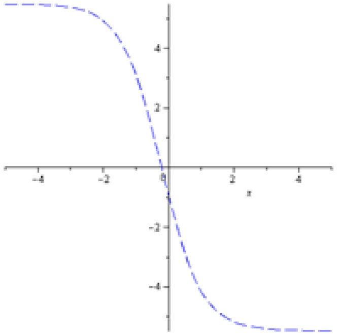
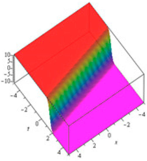
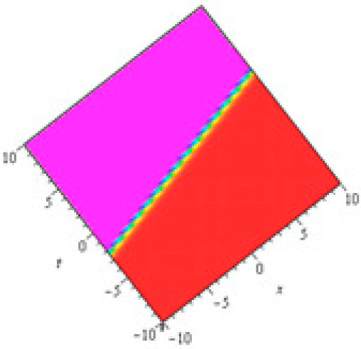
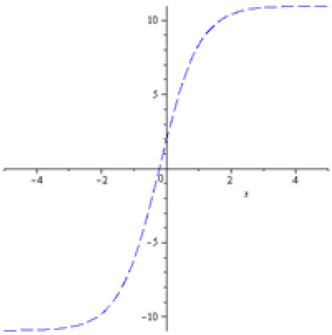
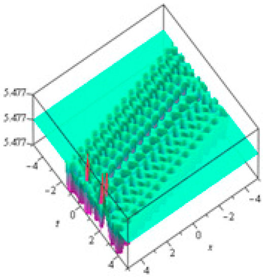
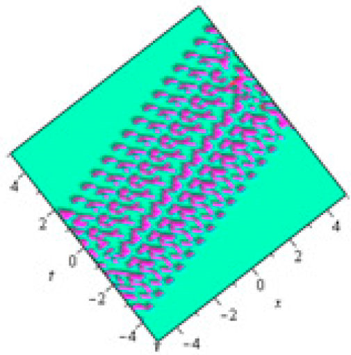
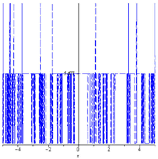
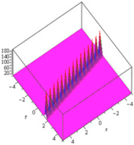
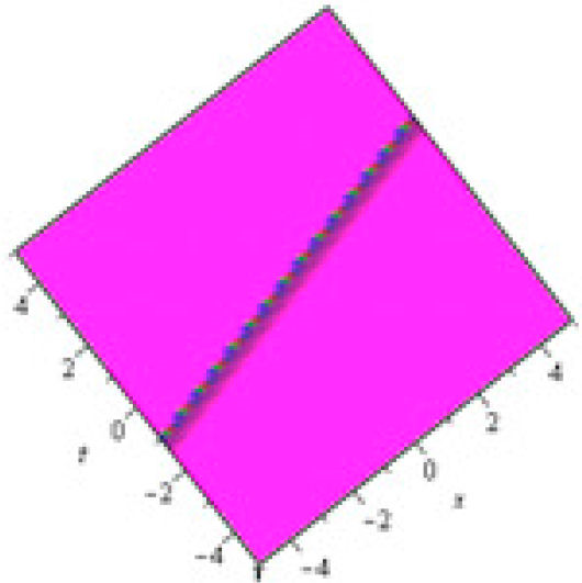
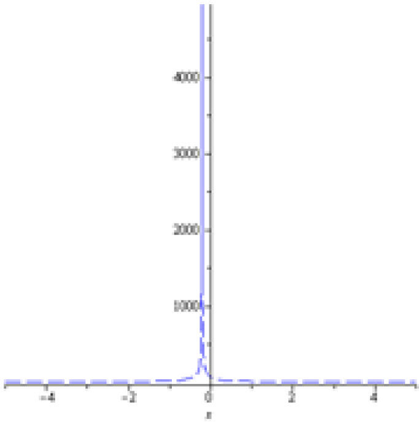
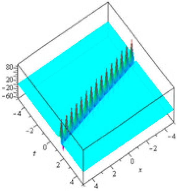
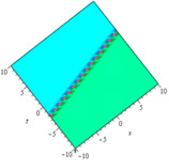
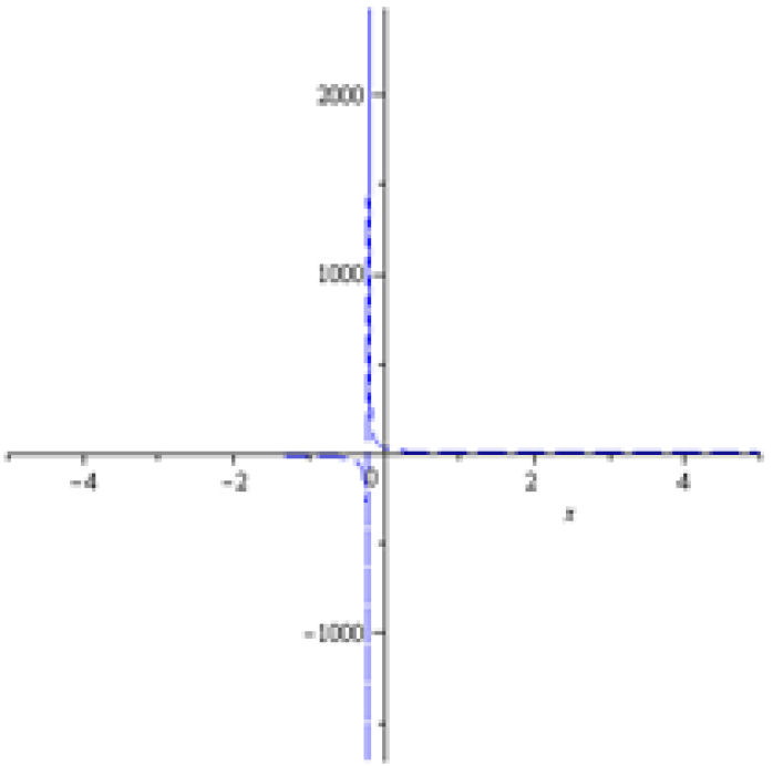
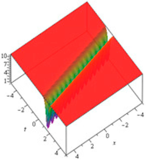
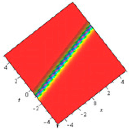
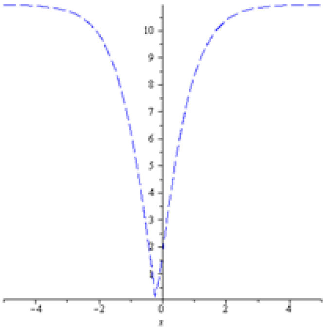
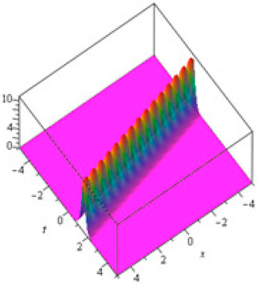
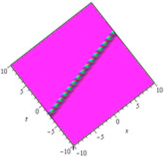
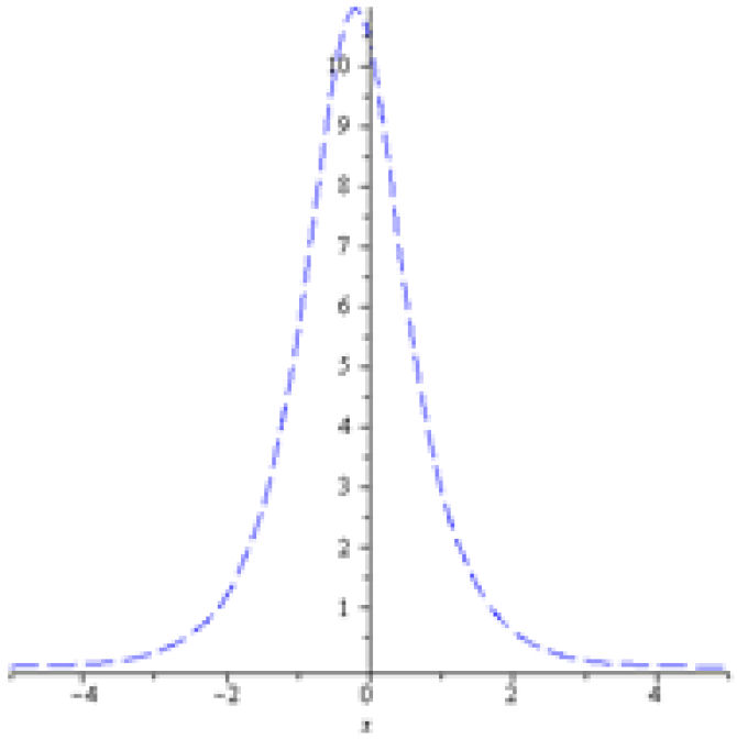
4 Figures and discussion of the solutions

In this section, we have plotted the graphs of the solitary wave solutions. At the moment, we assigned a set of appropriate values to obtain different soliton structures. Moreover, for the Sardar sub-equation solutions, and also for justification, we used β=1,  a=0.1,  b=2,  c=4,b1=4,β1=β3=1, β2=-0.5, and C = 1 uniformly to plot Figs. 1-5. Similarly, for the solutions derived via Ricatti, we β=1,  a=0.1,  b=2,  c=4,b1=4,β1=β3=1, β2=-0.5, ρ=1, and C = 1. We finally derived the following soliton structures.

Figure 1 The 3D plot of   Reu2±x,t

Figure 2 The contour plot of   Reu2±x,t.  

Figure 3 The 2D plot of   Reu2±x,t

Figure 4 The 3D plot of Reu13±x,t

Figure 5 The contour plot of Reu13±x,t

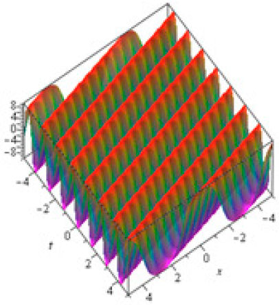
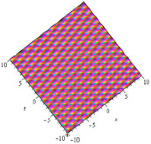
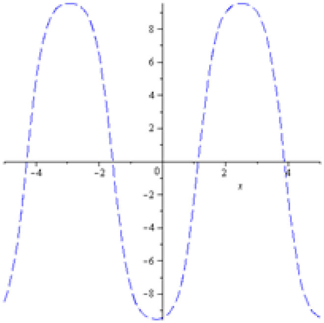
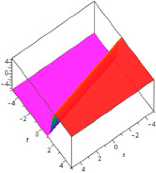
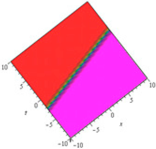
The recovered soliton structures in Figs. 1-24 for both approaches included singular, dark, bright, kink, anti-kink, and mixed solitons. For example, u1(x,t) and u2(x,t) correspond to kink soliton solutions, u3(x,t) corresponds to bright soliton solution, u5(x,t) and u17(x,t) correspond to dark soliton solutions, u6(x,t) and u18(x,t) correspond to singular soliton solutions, u7(x,t) and u19(x,t) correspond Bright-dark soliton solutions, u9(x,t) and u12(x,t) correspond dark-singular soliton solutions, and u10(x,t) corresponds to periodic soliton solutions. The structures in Figs. 1-8 are extremely useful in mathematical physics. Similarly, the same structures and beyond can be obtained using the appropriate values on the solutions derived via the two improved methods.

Figure 6 The 2D plot of Reu13±x,t

Figure 7 The 3D plot of Reu6±x,t.  

Figure 8 The contour plot of Reu6±x,t.  

Figure 9 The 2D plot of Reu6±x,t.  

Figure 10 The 3D plot of u15±x,t

Figure 11 The contour plot of u15±x,t.  

Figure 12 The 2D plot of u15±x,t

Figure 13 The 3D plot of u16±x,t

Figure 14 The contour plot of u16±x,t

Figure 15 The 2D plot of u16±x,t

Figure 16 The 3D plot of Reu12±x,t.  

Figure 17 The contour plot of Reu12±x,t.  

Figure 18 The 2D plot of Reu12±x,t.  

Figure 19 The 3D plot of u17±x,t.  

Figure 20 The contour plot of u17±x,t.  

Figure 21 The 2D plot of u17±x,t.  

Figure 22 The 3D plot of Imu24±x,t.  

Figure 23 The contour plot of Imu24±x,t.  

Figure 24 The 2D plot of Imu24±x,t[/p]  

5 Conclusion

In this paper, we categorically emphasized the effectiveness and generality of the two well-known, well-established, and classified techniques. Therefore, we employed the improved and modified Sardar sub-equation approach and improved generalized Riccati equation mapping method to investigate and analyze the new formats of exact solutions to the nonlinear improved mKdV equation. The techniques have been incorporated gently and applied to this well-known equation. However, the set of solutions, obtained by these techniques, has multiple and popular types of the form, i.e. rational, exponential, trigonometric, and trigonometric hyperbolic solutions of the improved mKdV equation. The methods are quick and highly effective in nature, whereas, in the first phase, we used the wave variable to transform the NPDEs into nonlinear ordinary differential equations (ODEs) with integer order after adapting the most general and simple techniques the IMSSEM and IGREMM are used to construct the novel solutions of the improved mKdV equation. Our findings imply that the approach is a strong, well-defined algorithm that is exceedingly efficient. It is confirmed from the profiles (soliton structures for both approaches) that the novel solutions preserved the qualities of singular, dark, bright, kink, anti-kink, and mixed solitons. Therefore, these methods applicable to solve various nonlinear PDEs arise in different areas of research and soliton. Additionally, these results may be helpful in the KdV equations family and application in engineering and mathematical science. We also presented a direct-viewing analysis by providing both two-dimensional and three-dimensional solution figures. Future studies will also concentrate on several fascinating findings connected to the suggested model, such as the physical feasibility, modulational stability, and the analysis of the lie symmetry of the solutions.

Acknowledgments

The authors would like to extend their sincere appreciation to the Researchers Supporting Project number (RSPD2024R802), King Saud University, Riyadh, Saudi Arabia.

References

[1] A. M. Wazwaz, The tanh-coth method for solitons and kink solutions for nonlinear parabolic equations, Appl. Math. Comput. 188 (2007) 1467, https://doi.org/10.1016/j.amc.2006.11.013. [ Links ]

[2] A. M. Wazwaz, The tanh-coth method for new compactons and solitons solutions for the K (n,n) and the K (n+1, n+1) equations, Appl Math. Comput. 188 (2007) 1930, https://doi.org/10.1016/j.amc.2006.11.076. [ Links ]

[3] A. M. Wazwaz, The sine-cosine method for obtaining solutions with compact and noncompact structures, Appl. Math. Comput. 159 (2004) 559, https://doi.org/10.1016/j.amc.2003.08.136. [ Links ]

[4] A, M. Wazwaz, A sine-cosine method for handling nonlinear wave equations, Math. Comput. Model. 40 (2004) 499, https://doi.org/10.1016/j.mcm.2003.12.010. [ Links ]

[5] N. Raza, M. R. Aslam, H. Rezazadeh, Analytical study of resonant optical solitons with variable coefficients in Kerr and non-Kerr law media, Optic Quant Electron. 51 (2019) 59, https://doi.org/10.1007/s11082-019-1773-4. [ Links ]

[6] N. Raza, A. Javid, Optical dark and dark-singular soliton solutions of (1+2) dimensional chiral nonlinear Schrodinger’s equation, Waves Random Comp Media. 29 (2019) 496, https://doi.org/10.1080/17455030.2018.1451009. [ Links ]

[7] M. M. Khater, A. R. Seadawy, D. Lu, Dispersive optical soliton solutions for higher order nonlinear Sasa-Satsuma equation in mono mode fibers via new auxiliary equation method, Serlattices Microstruct. 113 (2018) 346, https://doi.org/10.1016/j.spmi.2017.11.011. [ Links ]

[8] H. Rezazadeh, A. Korkmaz, M. Eslami, S. M. Mirhosseini-Alizamini, A large family of optical solutions to Kundu-Eckhaus model by a new auxiliary equation method, Optic Quant Electron. 51 (2019) 84, https://doi.org/10.1007/s11082-019-1801-4. [ Links ]

[9] E. C. Aslan, M. Inc, Optical soliton solutions of the NLSE with quadratic-cubic Hamiltonian perturbations and modulation instability analysis, Optik. 196 (2019) 162661, https://doi.org/10.1016/j.ijleo.2019.04.008. [ Links ]

[10] Z. Korpinar, M. Inc, M. Bayram, M. S. Hashemi, New optical solitons for Biswas- Arshed equation with higher order dispersions and full nonlinearity. Optik. 206 (2019) 163332, https://doi.org/10.1016/j.ijleo.2019.163332. [ Links ]

[11] I. K. Muhammad, A. Saleem, S. Jamilu, Jacobi Elliptic Function Expansion Method for the Improved Modified kortwedge-de Vries equation, Optical and Quantum Electronics 54 (2022) 734, https://doi.org/10.1007/s11082-022-04109-5. [ Links ]

[12] J. Sabi’u, A. Jibril, A. M. Gadu, New exact solution for the (3+ 1) conformable space-time fractional modified Korteweg-de-Vries equations via Sine-Cosine Method. Journal of Taibah University for Science, 13 (2019) 91, https://doi.org/10.1080/16583655.2018.1537642. [ Links ]

[13] G. Tao, J. Sabi’u, S. Nestor, R. M. El-Shiekh, L. Akinyemi, E. Az-Zo’bi, G. Betchewe, Dynamics of a new class of solitary wave structures in telecommunications systems via a (2+ 1)-dimensional nonlinear transmission line. Modern Physics Letters B, 36 (2022) 2150596, https://doi.org/10.1142/S0217984921505965. [ Links ]

[14] A. M. Wazwaz, The Hirota’s direct method and the tanh-coth method for multiple-soliton solutions of the Sawada-Kotera-Ito seventh-order equation, Appl Math Comput. 199 (2008) 133, https://doi.org/10.1016/j.amc.2007.09.034. [ Links ]

[15] A. M. Wazwaz, The Hirota’s direct method for multiple-soliton solutions for three model equations of shallow water waves, Appl Math Comput. 201 (2008) 489, https://doi.org/10.1016/j.amc.2007.12.037. [ Links ]

[16] W. Gao, H. Rezazadeh, Z. Pinar, H. M. Baskonus, S. Sarwar, G. Yel, Novel explicit solutions for the nonlinear Zoomeron equation by using newly extended direct algebraic technique, Optic Quant Electron. 52 (2020) 1, https://doi.org/10.1007/s11082-019-2162-8. [ Links ]

[17] H. Rezazadeh, New solitons solutions of the complex Ginzburg Landau equation with Kerr law nonlinearity, Optik. 167 (2018) 218, https://doi.org/10.1016/j.ijleo.2018.04.026. [ Links ]

[18] A. Yusuf, M. Inc, A. I. Aliyu, D. Baleanu, Optical solitons possessing beta derivative of the Chen-Lee-Liu equation in optical fiber, Front Phys. 7 (2019) 34, https://doi.org/10.3389/fphy.2019.00034. [ Links ]

[19] A. Yusuf, M. Inc, D. Baleanu, Optical solitons with M-truncated and beta derivatives in nonlinear optics. Front Phys. 7 (2019) 126, https://doi.org/10.3389/fphy.2019.00126. [ Links ]

[20] Y. Çenesiz, O. Tasbozan, A. Kurt, Functional Variable Method for conformable fractional modifed KdV-ZK equation and Maccari system, Tbilisi Math J. 10 (2017) 117, https://doi.org/10.1515/tmj-2017-0010. [ Links ]

[21] M. Eslami, H. Rezazadeh, M. Rezazadeh, S. S. Mosavi, Exact solutions to the space-time fractional Schrödinger-Hirota equation and the space-time modifed KDV-Zakharov-Kuznetsov equation, Optic Quant Electron. 49 (2017) 279, https://doi.org/10.1007/s11082-017-1112-6. [ Links ]

[22] S. Nestor, A. Houwe, H. Rezazadeh, A. Bekir, G. Betchewe, S. Y. Doka, New solitary waves for the Klein-Gordon-Zakharov equations, Modern Phys Lett B. 60 (2020) 324, https://doi.org/10.1142/S0217984920502462. [ Links ]

[23] A. Houwe, J. Sabi’u, G. Betchewe, M. Inc, S. Y. Doka, Modulation analysis and optical solitons of perturbed nonlinear Schrödinger equation. Rev. Mex. Fis. 67 (2021) 040705, https://doi.org/10.31349/RevMexFis.67.040705. [ Links ]

[24] S. Nestor, S. Abbagari, A. Houwe , G. Betchewe , S. Y. Doka , Diverse chirped optical solitons and new complex traveling waves in nonlinear optical fibers, Commun Theor Phys. 72 (2020) 065501, https://doi.org/10.1088/1572-9494/ab7ecd. [ Links ]

[25] A. Houwe , S. Abbagari , M. Inc , G. Betchewe , S. Y. Doka , Crépin, et al. Chirped solitons in discrete electrical transmission line, Results Phys. 18 (2020) 103188, https://doi.org/10.1016/j.rinp.2020.103188. [ Links ]

[26] C. Park et al., Dynamical analysis of the nonlinear complex fractional emerging telecommunication model with higher-order dispersive cubic quintic, Alexandria Eng J. 59 (2020) 1425, https://doi.org/10.1016/j.aej.2020.03.046. [ Links ]

[27] M. Alquran, A. Jarrah, Jacobi elliptic function solutions for a two-mode KdV equation, J. King Saud Univ Sci. 31 (2019) 485, https://doi.org/10.1016/j.jksus.2017.06.010. [ Links ]

[28] H. M. Jaradat, M. Syam, M. Alquran, A two-mode coupled Korteweg-de Vries: multiple-soliton solutions and other exact solutions, Nonlinear Dyn. 90 (2017) 371, https://doi.org/10.1007/s11071-017-3668-x. [ Links ]

[29] M. Alquran, H. M. Jaradat , M. I. Syam, A modified approach for a reliable study of new nonlinear equation: two-mode Korteweg-de Vries-Burgers equation, Nonlinear Dyn. 91 (2018) 1619, https://doi.org/10.1007/s11071-017-3968-1. [ Links ]

[30] H. M. Jaradat , F. Awawdeh, S. Al-Shara, M. Alquran ,S. Momani, Controllable dynamical behaviors and the analysis of fractal burgers hierarchy with the full effects of inhomogeneities of media, Rom. J. Phys. 60 (2015) 324. [ Links ]

[31] M. Syam, H. M. Jaradat , M. Alquran , A study on the two-mode coled modified Korteweg-de Vries using the simplified bilinear and the trigonometric-function methods, Nonlinear Dyn. 90 (2017) 1363, https://doi.org/10.1007/s11071-017-3732-6. [ Links ]

[32] M. Alquran , H. M. Jaradat , S. Al-Shara, F. Awawdeh, A new simplied bilinear method for the N-soliton solutions for a generalized F mKdV equation with time-dependent variable coefficients, Int J Nonlinear Sci Numer Simul. 16 (2015) 259, https://doi.org/10.1515/ijnsns-2014-0023. [ Links ]

[33] H. Rezazadeh, J. Vahidi, A. Zafar, A. Bekir, The functional variable method to find new exact solutions of the nonlinear evolution equations with dual-power-law nonlinearity, Int J Nonlinear Sci Numer Simul. 21 (2020) 249, https://doi.org/10.1515/ijnsns-2019-0064. [ Links ]

[34] H. Yépez-Martínez, J. F. Gómez-Aguilar , Fractional sub-equation method for Hirota-Satsuma-coled KdV equation and coled mKdV equation using theAtangana’s conformable derivative, Waves Ran. Comp. Med. 29 (2019) 678, https://doi.org/10.1080/17455030.2018.1464233. [ Links ]

[35] J. Sabi’u , M. Inc , T. D. Leta, D. Baleanu, H. Rezazadeh, Dynamical behaviour of the Joseph-Egri equation. Thermal Science, 27 (2023) 19, https://doi.org/10.2298/TSCI23S1019S. [ Links ]

[36] H. Yépez-Martínez, J. F. Gómez-Aguilar, M-derivative applied to the soliton solutions for the Lakshmanan-Porsezian-Daniel equation with dual-dispersion for optical fibers, Optical Quant Electron. 51 (2019) 31, https://doi.org/10.1007/s11082-018-1740-5. [ Links ]

[37] L. Akinyemi, Two improved techniques for the perturbed nonlinear Biswas-Milovic equation and its optical solutions, Optik 243 (2021) 167477, https://doi.org/10.1016/j.ijleo.2021.167477. [ Links ]

Received: October 25, 2022; Accepted: April 08, 2023

Creative Commons License This is an open-access article distributed under the terms of the Creative Commons Attribution License