1. Introduction

Cancer is a major frequent public health issue that imposes a significant burden. Not only is it widespread over the world, but the World Health Organization (WHO) predicts that by 2030, 27 million additional cancer cases would have been diagnosed (^{International Agency for Research on Cancer, 2008}). There are many different forms of cancer, such as skin cancer, prostate cancer, colon cancer, blood cancer (^{Hassanpour & Dehghani, 2017}), and so on. Breast cancer is the second most frequent cancer in women after skin cancer, making it one of the most common cancer kinds. Unfortunately, among the cancer forms, breast cancer (BC) has the highest mortality rate (^{Hassanpour & Dehghani, 2017}).

Although there are various approaches for detecting BC, including molecular biology in the search for novel BC markers, histopathology examination is currently the most often used method (^{International Agency for Research on Cancer, 2012}). Pathologists often analyze histology specimens under a microscope to assess the stage and grade of breast cancer. However, as technology progresses, image processing tools and machine learning approaches have made it feasible to construct computer-aided systems that can categorize tissue samples and detect the presence of cancer. The major purpose of a cancer-computer-aided detection system is to correctly classify cancer, but the intricacy of histology pictures makes successful classification difficult (^{Stenkvist et al., 1978}). However, utilizing machine learning approaches like neural networks and support vector machines (SVM), several research were able to generate outcomes with high accuracy ranging from 76% to 94 percent (^{George et al., 2014}).

Convolutional neural network (CNN) is widely used among the different machine learning algorithms to get state-of-the-art results in pattern recognition (^{Krizhevsky et al., 2017}; ^{LeCun et al., 1989}; ^{Niu & Suen, 2012}). Similarly, a study has shown that CNN can readily outperform classical descriptors in picture texture classification for both microscopic and macroscopic textures (^{Hafemann et al., 2014}).

Some of the most well-known research on breast cancer categorization relies heavily on the whole slide imaging (WSI) method (^{Doyle et al., 2008}; ^{Kowal et al., 2013}; ^{Zhang et al., 2013}; ^{Zhang et al., 2014}). These solutions, on the other hand, face obstacles such as high implementation costs, unresolved regulatory difficulties, and inherent technological concerns (^{Evans et al., 2015}). Furthermore, until Spanhol et al. (2016) provided a big dataset made up of 7909 images obtained from 82 individuals, most research relied on limited datasets including histological samples. Also, they evaluated the effectiveness of six textural descriptors as well as different classifiers in their investigation, obtaining findings with an accuracy of 80 to 85 percent. Regardless, some researchers believe that the feature engineering stage is where machine learning approaches fail (^{Bengio et al., 2013}; ^{LeCun et al., 2015}). ^{Sheikh et al. (2020)} introduced the (MSI-MFN) technique for breast cancer classification, which relies on multi-scale input and multi-feature networks. They used two public datasets for evaluating the model, the first dataset is ICIAR2018 which contains 400 stained images (2048 × 1536 pixels), the second dataset is BreakHis which contains 7909 samples, each categorized as either benign or malignant. The subsets of benign and malignant samples contain 2480 and 5429 samples (700 × 460 pixels). The approach extracts more relevant and diversified characteristics by merging multi-resolution feature maps derived from the dense connective structure of the network utilizing four separate layers. The system can learn the textures of the cells as well as their general structure after training multiple picture patches. The suggested system consists of a pre-processing step that comprises multi-scale input, a training stage that involves data augmentation, and a testing stage that generates more patches. Following that, the processing step takes place, which involves a lot of concatenation. As a result, the CNN algorithm is used in the categorization. On two datasets, the performance of this strategy was assessed, and it outperformed state-of-the-art models in terms of accuracy, specificity, and sensitivity. ^{Zhu et al. (2019)} proposed using several compact CNNs to classify breast cancer via histological pictures. More specifically, the system uses hybrid CNN architecture to provide a stronger representation capability. This is made feasible by combining information from two branches and local voting. A channel pruning module is also utilized to make the network more compact, in addition to combining two model branches. The benefits of the proposed model may be summarized as the ability to achieve improved accuracy while utilizing the same model size. Furthermore, the problem of over-fitting is not an issue with this model. The proposed model can deliver results like state-of-the-art models when evaluated on the BreaKHis dataset. The researchers then proceeded to assemble a variety of models to improve the performance of the recommended model. The multi-model strategy beat state-of-the-art models in terms of picture level and patient level accuracy on the BACh dataset. ^{Jiang et al. (2019)} formed a novel convolutional network which included a convolutional layer, a small SE-ResNet module, and a completely linked layer. BHCNET was the proposed model's name. To decrease the network's parameters, the tiny SE-ResNet module is employed. Furthermore, when compared to the bottleneck SE-ResNet, the parameters were reduced by 29.4 percent, and 33.3 percent when compared to the basec SE-ResNet. The researchers also created the Gauss error scheduler, which is a learning rate scheduler that gives the user more latitude rather than fine-tuning the SGD algorithm's learning rate parameter. When the suggested strategy was evaluated on binary classification, the model achieved accuracy levels of 98.87 percent to 99.34 percent. In multi-classification, however, the model achieved accuracy values of 90.66 percent to 93.81 percent.

CNN is a neural network that has an interconnected structure. The CNN method is one of the popular deep learning methods that form convolutional operations on raw data (^{Alom et al., 2019}). It has been applied in various applications such as speech recognition, sentence modeling, image classification and, recently, medical imaging, including breast cancer diagnosis. Three layers make up CNN: a convolutional layer, a pooling layer, and a fully connected layer. These layers are stacked to create a deep architecture for automatically extracting the features (^{Alom et al., 2019}). Recently, several of the CNN models have been introduced by different researchers: VGG (^{Zhao, Zhang, et al., 2022}), AlexNet (^{Zhao, Hu, et al., 2022}) and GoogleNet (^{Binder et al., 2016}).

RNN is a supervised deep learning-based technique used for sequential data (^{Mambou et al., 2018}). The hidden unit of the recurrent cell is used by RNN to learn complex changes by integrating a temporal layer for capturing sequential information (^{Yao et al., 2019}). Depending on the information accessible to the network, which is automatically updated to represent the network’s current state, the hidden unit cells may change (^{Mambou et al., 2018}). However, the model suffers from vanishing or exploding gradients and is difficult to train, which limits its application for modeling temporal dependencies and longer sequences in a dataset (^{Egger et al., 2022}). To mitigate the issue of the vanishing and exploding gradients of RNN, new models such as long short-term memory (LSTM) and gated recurrent unit (GRU) were introduced (^{Hossain et al., 2019}). To manage the flow of information into the network, LSTM included memory cells to store relevant data (^{Nasser & Yusof, 2023}). The LSTM can represent temporal dependencies and effectively capture the global features in sequential data to improve the speed (^{Egger et al., 2022}). However, one of the problems of the LSTM is the issue of the numerous parameters that are required to be updated during the model training (^{Nasser & Yusof, 2023}). To reduce the parameter update, the GRU with fewer parameters, which makes it faster and less complicated, is introduced. The next hidden state’s updating process and contents exposure technique are different for LSTM and GRU (^{Schmidhuber, 2015}). While GRU updates the subsequent hidden states based on the correlation, subject to the amount of time required to maintain such information in the memory, the LSTM updates the hidden states using the summing operation.

The performance of deep learning in the categorization of breast cancer in histological images is evaluated in this work by using CNN on a large dataset. The suggested model's performance will also be compared to that of other methods utilizing the same dataset.

The following sections will describe the structure of the proposed CNN network and the layers present in it, along with an explanation of the function of each layer. The data set and the data preparation process will also be described, after which performance measures will be discussed and conclusions drawn and discussed.

2. Materials and methods

This section goes through some of the most significant aspects that went into making our suggested CNN model work. This section also provides a detailed account of the materials, data, and methods used in the study. It includes information about the dataset used, data preprocessing techniques, the architecture of the neural network, training parameters, evaluation metrics and the experimental setup.

CNN Architecture gets their name from the fact that they have convolutional layers in their design. convolutional layers are mostly used to detect visual characteristics. CNN learns a characteristic of an image with each movement of the kernel on the picture. Each neuron in the convolutional layer is utilized to extract characteristics from an image's tight structure. The weights of each neuron are shared amongst the nodes in the convolutional layers to acquire comparable features for the input picture channels.

The first layer of a deep convolutional neural network is trained by feeding it data and allowing it to calculate and extract the feature before generating the output. The error is estimated after the output is computed, and this error is transmitted backward across the network via back-propagation. Parameters are fine-tuned at each phase of the model to reduce error. This method keeps on with the data and improves the model as it goes. The input is supplied to these levels, and parameters are updated in each layer until the model converges. Training the CNN is an iterative process that includes many layers, and the input is sent to these layers and parameters are updated in each layer until the model converges. Convolutional neural network architecture is made up of three layers: the convolutional layer, the fully connected layer, and the pooling layer. In general, a completely CNN architecture is constructed by stacking multiple of these layers one on top of the other. Figure 1 shows a general example of CNN architecture.

Figure 1 Flowchart of CNN architecture. 

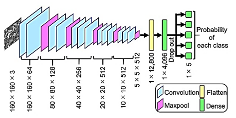
Extraction of a feature from a picture or image is the primary calculation of CNN. The image is sent into the convolution layer, along with a tiny kernel that is moved around the image. Each pixel of an image and a kernel or filter is used to construct a dot product. A kernel, sometimes known as a convolution kernel, is a collection of common weights.

Assuming that an image is 512 × 512 pixels in size, an image kernel or filter may be (3 × 3, 5 × 5, or 8 × 8) in size, and each neuron is linked to these filters or solely to this section of the image in a previous layer. As a result, a convolutional kernel learns to recognize the feature of a picture or image that is evident in the feature map. Each grouping of convolution layers is followed by a pooling layer; a work procedure evocative of straightforward and complicated cells in the important visual cortex [4] to reduce computational multifarious nature and achieve a diverse leveling collection of image contains (^{Krizhevsky et al., 2017}). By picking the relevant feature and constructing a feature map for each picture, the maximum pooling layer is utilized to minimize the size of the image. The low-level feature value is discarded while using max pooling, but the high-level feature value is kept in the feature vector. As a result, max pooling may improve translation invariance as well. A few sets of convolutional, rectified linear unit (ReLU), pooling layers, and completely linked layers are typically used in CNNs (^{Evans et al., 2015}). Between two convolutional layers, a pooling layer may be placed. The primary purpose of adding pooling layers between convolutional layers is to minimize the image's spatial size. As a result, it aids in reducing the amount of parameters and computations required by the neural network, hence reducing over-fitting. The pooling (sub sampling) layer spatially down samples the picture volume and is independent in each input volume depth slice. Figure 2 shows the layered structure used in the proposed CNN.

Figure 2 The layered structure used in the proposed CNN. 

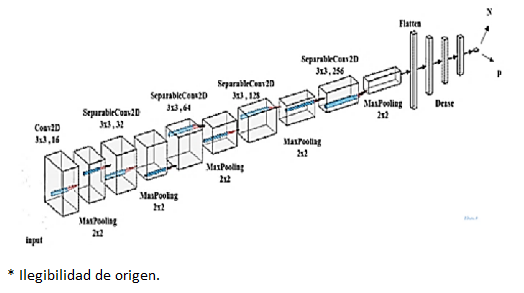
The previous figure provides a comprehensive view of the proposed architecture, and what the outputs look like after the operations of each layer. This architecture is designed with a combination of convolutional, pooling, normalization, and fully connected layers to capture and process features effectively. The presence of dropout and BatchNormalization indicates a focus on addressing overfitting and improving training stability.

The CNN is configured to process inputs of size (224,224,3) by passing the parameter shape = (224,224,3) to the first layer.

Conv2D layers are used for a convolution operation that extracts features from the input images by moving the convolution filter over the input images to produce map features. In our model, 16 filters with a window size of 3x3 are selected.

SeparableConv2D layers are used for a process in which one convolution can be split into two or more convolutions to produce the same output. One process is divided into two or more subprocesses to achieve the same effect. Here we choose 32 filters with a window size of 3x3 for the first two groups, 64 filters for the second two groups, 128 for the third group of two groups, and 256 for the last two groups.

Max pooling layers are used for a max pooling process that reduces the dimensionality of each feature, which helps shorten training time and reduce the number of parameters. A (2 × 2) pooling window was chosen.

To combat overfitting, dropout layers, a powerful organizing technique, were used. It forces the model to learn multiple independent representations of the same data by randomly deactivating neurons in the learning phase. For example, layers will randomly disable 20% of the output in all groups.

Finally, we use flatten to reduce the image dimensions to 1D and add 3 fully connected dense layers. The dense layer processes 1D image vectors for output.

The previous network structure was reached based on the experimental results, where the training process is conducted, and the model’s performance is verified. If the performance is low, the network structure is modified and retrained, and so on until the proposed network structure that was clarified, and which achieved the best performance based on the experimental results was reached.

2.1. BreaKHis database

The BreaKHis database, which has a collection of microscopic pictures of both benign and malignant breast tumors and is separated into two groups for training (70 %) and testing (30 %) in accordance with the experimental procedures, was selected to be used in this investigation. The data set is divided such that the training set is not utilized for testing, allowing the algorithm to accurately categorize the unseen patient image (^{Benhammou et al., 2020}).

Assume that N: is the total number of cancer images of the test data, and N_rec: is the images which truly classified. So, the classification accuracy can be given as in Eq. 1.

Accuracy=NrecN×100 (1)

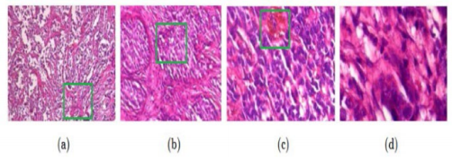
We utilized a magnification factor of 400 in our study, and the images were split as follows: There are 1146 photographs of malignant breast tumors and 547 images of benign breast tumors (see Figure 3).

Figure 3 Breast malignant tumor slides observed with different magnification ratios (a) ×40, (b) ×100, (c) ×200 and (d) ×400. 

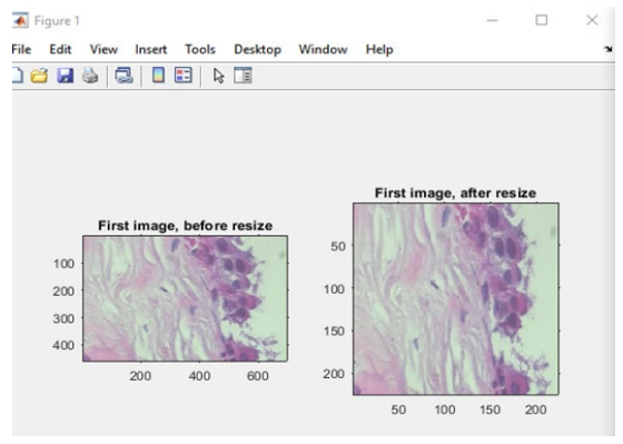
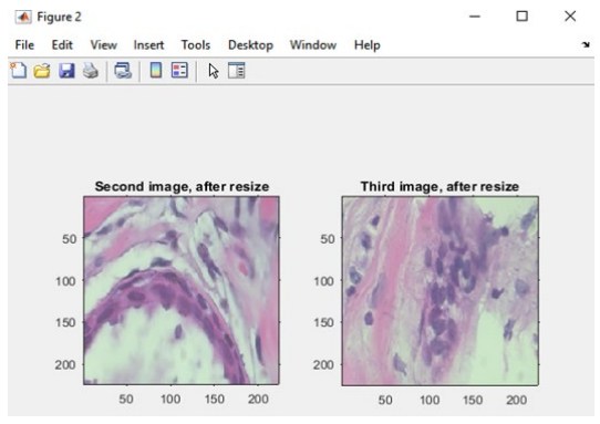
2.2. Data preparation

The sizes of the photographs were changed during the data preparation process to ensure that they were all the same size. Furthermore, the photos in the dataset were divided into benign and malignant categories and placed in different files (see Figure 4 and Figure 5). We used to resize() instruction in MATLAB R2019a in this process.

Figure 4 Image before and after resizing. 

Figure 5 All images in the dataset are resized. 

3. Results and discussion

After the completion of the training phase, the accuracy of our proposed model was calculated in addition to the loss function.

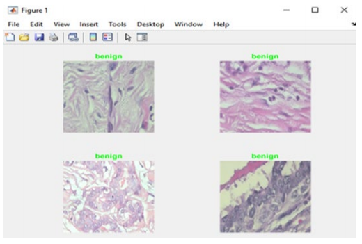
The proposed model was evaluated on a group of randomly chosen images, and the result of the classification was compared to the original labeling (benign or malignant). Whenever the model achieves the right classification prediction, the label of the respective image will be in green. On the other hand, if the classification prediction if wrong, the label of the respective image will be in red.

We designed a graphical user interface GUI using MATLAB to make it easier to run the software and display the results. Figure 6 depicts the intended user interface.

Figure 6 GUI was designed in this study. 

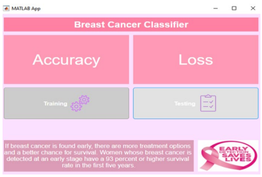
As can be seen in Figure 6, the GUI enables the viewing of the proposed system's accuracy and loss numbers.

Figure 6 shows the accuracy, loss, training, and testing tabs which described as follows:

1. Accuracy: Accuracy is a metric used to evaluate the performance of a machine learning or deep learning model. It measures the proportion of correctly classified instances out of the total instances in the dataset. It is often expressed as a percentage and is a common way to assess the model's overall correctness in its predictions.

2. Loss: Loss, also known as a loss function or cost function, is a measure of the error or dissimilarity between the predicted output of a model and the actual target values in the dataset. The goal during training is to minimize this loss, as a lower loss indicates better alignment between the model's predictions and the ground truth.

3. Training: In the context of machine learning, training refers to the process of fitting a model to a dataset. During training, the model learns to make predictions by adjusting its internal parameters based on the provided data and minimizing the loss function. Training involves iterating through the dataset multiple times (epochs) and updating the model's parameters through techniques like gradient descent.

4. Testing: Testing, in the context of machine learning, involves assessing the model's performance on a separate dataset that it has not seen during training. This dataset, called the test set, is used to evaluate how well the model generalizes to new, unseen data. Metrics like accuracy, precision, recall, and F1-score are often calculated on the test set to determine the model's effectiveness and generalization capability.

Figure 7 shows a sample of the findings, showing that the algorithm properly identified four images (all of which were benign), and so their labels appear in green.

Figure 7 Correct classification of breast tumors in histopathological samples. 

Similarly, Figure 8 shows that the obtained accuracy is 84.9, whereas the loss value is 0.15.

Figure 8 Accuracy and loss values by experimentation. 

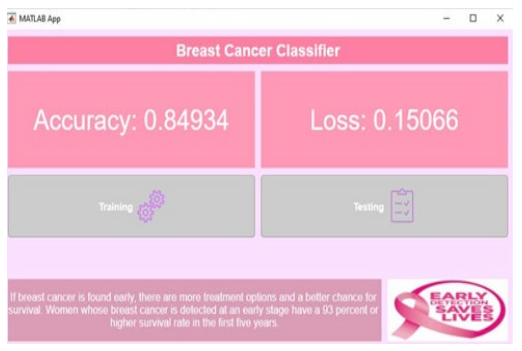
An accuracy of 0.84934 and a loss of 0.15066 indicate a satisfactory performance for a convolutional neural network (CNN) in cancer detection:

1. Accuracy: An accuracy of 84.93% is a solid result, especially in the context of medical image analysis. It means that the model correctly predicts cancer in 85% of cases. However, the clinical significance depends on the specific use case. In some medical applications, even higher accuracy may be required.

2. Loss: A low loss value of 0.15066 indicates that the model's predictions are close to the actual values, which is a positive sign. Lower loss values imply a well-trained model.

3. Data and generalization: It is crucial to consider the quality and quantity of the dataset used for training. If the dataset is representative and large enough, it can enhance the model's ability to generalize to unseen cases. Additionally, it is essential to evaluate the model on an independent test dataset to ensure it does not overfit the training data. This can be considered as future work.

4. Conclusions

BC is one of the main public health concerns, particularly since it claims the lives of so many women each year. Because early diagnosis is so important in saving lives, it is crucial to develop models that can aid pathologists in the categorization process so that they can make accurate diagnoses. As a result, we suggested a strategy for the classification of BC in histopathological samples acquired from the BreaKHis dataset that uses a convolutional neural network. The findings reveal that our suggested system can accurately categorize photos from a large dataset with 73 percent accuracy.

The research focused on the role of convolutional neural networks (CNNs) in the detection of cancer, and the following key findings have been derived:

1. Performance evaluation: The CNN model achieved an accuracy of 84.93% and a low loss value of 0.15066, indicating a strong ability to correctly classify cancer cases.

2. Data quality and generalization: The research emphasizes the importance of a high-quality and representative dataset, as it significantly influences the model's performance and generalization to unseen cases.

3. Clinical significance: While the accuracy is promising, the clinical relevance of the model's performance depends on the specific medical application. Further evaluation in a clinical context is necessary to assess its real-world impact.

4. Interpretability: The research highlights the importance of model interpretability, particularly in medical diagnostics, to gain the trust of healthcare professionals and ensure the model's predictions are explainable. In the research, the model and the proposed network structure were explained accurately, along with the details of each layer and the benefits of using it.

In summary, the research demonstrates the potential of CNNs in cancer detection, with a strong emphasis on the need for data quality, clinical evaluation, and ethical considerations in the deployment of such models. Further investigations, improvements, and validation in clinical settings are recommended to advance the practical utility of the CNN-based approach in cancer diagnosis.