


 text new page (beta)
 English (pdf)
 Article in xml format
 Article references
 Send this article by e-mail
 Cited by SciELO
  Similars in
SciELO
Similars in
SciELO 
 Permalink
Introduction
The American bullfrog (Lithobates catesbeianus, Shaw, 1802) belongs to the Ranidae family and is among the most economically and ecologically relevant amphibian species in the world. This is firstly because it is commonly used in international cuisine (mainly in the United States, France, Belgium, Canada, Italy and Spain,1 but also as it has become one of the 100 most invasive species in the world,2 as a result of its worldwide expansion for aquaculture development (in over 40 countries).3 Commercial demand for American bullfrogs increased in the international market from the 1980s, pushing the need to develop and modernize existing production systems.7 The world bullfrog market has steadily grown since the 1990s,1 with China heading annual production, followed by Singapore and Malaysia, while Brazil and Mexico are fourth and fifth, respectively. In fact, production has increased considerably in several countries, reaching an average annual revenue of $28,141,319 US dollars in 2011.1 Bullfrog farming formally began in Mexico in 1925,4 and has since been introduced in at least 16 states, Michoacán having the higher production yield in the country.5,6 Since then, México has become an important bullfrog producer, especially for the American market, reaching over 202 tons and a production value of $18,960,792 Mexican pesos in 2015.4,6
Aquaculture is the fastest growing food industry in the world,8 partly due to the fact that fish and amphibians use energy more efficiently and have a better nutrient conversion into protein, when compared to conventional farm animal species.9 Nonetheless, the high annual genetic gains achieved in fish breeding programs (which are 5 to 6 times higher than in farm animals), have not been mirrored for bullfrog, or any other anuran species, farming.9 For instance, growth rate for Nile tilapia and Atlantic salmon was increased by 85% and 115% in only six generations, respectively.10 Moreover, information on productive traits such as weight, growth rate, disease resistance and survival under intensive farming conditions is almost non-existent in México.11,12 According to Gjedrem and Robinson,10 in order to develop a successful breeding program, it is necessary to first generate knowledge about phenotypic and genetic parameters for economically important traits. Therefore, the aim of the present study was to characterize a number of morphometric and physiological variables of American bullfrogs, bred under intensive production systems in Mexico.
Materials and methods
Farms
Five bullfrog farms located in three different states of Mexico were studied. Three of these farms are situated in the state of Michoacán, at La Purisima (LP, coordinates 19°52’11”N, 101°01’23”W; 1,800 m.a.s.l.) and Isla de Tzirio (TZI) communities (19°20’11”N, 99°49’79”W; 1,772 m.a.s.l.), both in the Álvaro Obregón municipality; and the third one in the Copuyo (COP) community (19°29’50.5”N, 100°55’56.1”W) within the Tzitzio (TZI) municipality (1,540 m.a.s.l.). The fourth farm (Aquanimals) is found in the state of Querétaro, within the municipality of Villa Corregidora (COR), (20°33’33.7”N, 100°27’26.0”W; 2,260 m.a.s.l.). Finally, the fifth farm is located in the State of Mexico, in San Pedro Tlaltizapan (SPT, 19°12’14.4”N, 99°30’02.8”W; 2,742 m.a.s.l.), within the Toluca municipality. All farms had intensive production systems, with cement tanks with an area of 2.5 m² approximately, which were placed inside greenhouses with conventional polyethylene covers. Animals were fed under ad libitum “semi-dry” conditions,1 using commercial food originally formulated for rainbow trout (either from the Purina brand in the Copuyo and Aquanimals farms, or El Pedregal brand in La Purísima, Isla de Tizirio and San Pedro Tlaltizapan farms). The Purina formulation provides 40-48% protein, 12% fat, 3% fiber, 14% humidity and 12% ash, whilst El Pedregal formulation supplies 45% protein, 16% fat, 2.5% fiber, 12% humidity and 12% ash. Temperature inside the greenhouses was controlled manually on a day-to-day basis, according to readings obtained from calibrated digital or analog thermometers.
Animals
Male and female frogs from two sexual maturation stages were used for the study. Three year old breeding adults (n = 100), which were designated as “breeders” came from all five of the above-mentioned farms, and were used solely for non-invasive linear morphometry and body condition studies, since producers would not allow for euthanasia of offspring-yielding individuals. In addition, sixty one-year-old juvenile frogs (age at which they reach commercial or harvest size), from the LP and SPT sites were used. Invasive analyses that required animal sacrifice were performed on this group. Juveniles were further divided to form four different groups according to locality and sex [female (F) or male (M); LP-F, LP-M, SPT-F, SPT-M; n = 60]. To minimize stress, juvenile frogs were kept in 200 liter capacity plastic containers during transport to the laboratory, which took no more than six hours. Once in the laboratory, frogs were kept in dark and quiet conditions for 12 hours before slaughter. All handling and experimentation procedures followed the International Guidelines for the use of animals in Biomedical Research, and complied with the official Mexican norm for care and use of laboratory animals (NOM-62-ZOO-1999).
Body condition
Body condition was determined through the scaled mass index (SMI), following the method previously described by Peig et al.18 This index is better than other condition indices (e.g., ordinary least square regression), because it has a greater correlation with fat reserves and muscle mass in mammals, reptiles and amphibians such as bullfrogs and newts (Taricha granulosa).13,14 The SMI value relates to the adjusted weight of each individual, according to the scaling factor bSMA determined for each group of frogs (see below). The SMI was calculated according to the following formula:
Where Mi indicates body mass and Li represents snout to vent length (SVL) of each individual. Lo is the arithmetic mean of the SVL values of the animals in each group, and bSMA is the slope of a standardized major axis regression of mass on SVL. Thus, for each of the juvenile bullfrog groups (two different localities and both sexes), the bSMA scaling exponent represents the linear relationship between weight and body length. If mass is perfectly correlated with body volume, as it would in an isometric relation, then a bSMA value of 3 would be expected. Animals that have a lower bSMA, have more mass in relation to length. Conversely, bSMA values above 3 mean that animals have less mass in relation to length. The bSMA value (which in itself provides information about body condition of a population) is also used to calculate the adjusted or scaled value of each frog’s weight, expressed in grams, that is called SMI.
Hematology
Hematological analyses were performed in one-year-old juvenile frogs from LP and SPT locations (n = 60). Immediately after decapitation, blood was collected from the trunk in EDTA containing tubes and stored at 4 °C. To calculate the hematocrit and obtain plasma, 2ml of blood was centrifuged at 4,500 rpm for 15 minutes. The proportion of erythrocytes was measured with a Vernier caliper. White blood cells (WBC) were stained following the Turk method (dilution of blood with Turk 1/100 reagent) and counted in a hemocytometer. The differential leukocyte calculation was carried out by counting 100 Wright hematoxylin stained cells on blood smears, under a bright field microscope (40×).
Linear morphometry
Multivariate morphometric analyses were performed on both breeder and juvenile bullfrogs, including individual weight (measured in grams), snout to vent length (SVL), head width, head length, eardrum diameter (taken perpendicular to the maxilla), eye diameter (measured through its longest axis), hind leg length (femur plus tibia and fibula), and foot length (tarsus and metatarsals). A Vernier caliper (margin of error 0.01 cm) was used for all linear measurements, and results were expressed in cm.
Geometric morphometry
Geometric morphometry analyses have been previously used to document the existence of phenotypic variability within the same amphibian species.15 First, hot water pre-treated male and female skulls from juvenile frogs were cleaned with a 5.4% sodium hypochlorite solution and then manually dissected. Ventral photographs of clean dissected skulls were subsequently taken, and ten anatomical landmarks established in each frame with the aid of the TpsUtil and Tps2 software (James Rohlf, Stony Brook University16) (Fig. 1A). These landmarks formed a set of Cartesian coordinates for each individual, with a distribution that captured morphologically distinct shape variables. Thus, variability of landmark coordinates among individuals reflects differences in the shape of anatomical structures. To contrast differences, the first step in the process was to define the landmark set to be used (Fig. 1A). It is important that chosen landmarks be consistent and anatomically recognizable in all specimens, and that they capture the shape of the structure that is to be analyzed. Selected landmarks for this study were: 1) the medial and dorsal limit of the parasphenoid bone, 2) the midpoint of the vomer bone at the height of the palatine process, 3) the outermost posterior point of the premaxilla, 4) the anterior end of the premaxilla at the edge of the skull, 5) the dorso-lateral end of the paraesphenoid bone, 6) the parasphenoid bone and pterygoid plate union, 7) the premaxillary-maxillary suture, 8) the posterior end of the pterygoid-quadratojugal joint, 9) the converging point between the pterygoid plate and the maxilla, and 10) the palatine process of the maxilla union (Fig. 1A). All these landmarks where validated in previous studies where ontogeny and phylogeny of ranid frogs (including bullfrogs) was investigated.17,18 The landmark coordinates of frogs within each group of juveniles (i.e. SPT-F, LP-F, SPT-M, and LP-M) were superimposed by a method called Procrustes alignment (Fig. 1B). This method allows for the removal of intra-group variation of size, position and orientation from the resulting superimposed landmarks. Final coordinates for the superimposed landmarks were next incorporated to a canonical variate analysis (explained below), to visualize data and test for differences between groups (for a detailed technical explanation of the procedure, see Klingenberg19). The Procrustes alignment and subsequently MorphoJ software were used to assess geometric morphometry.
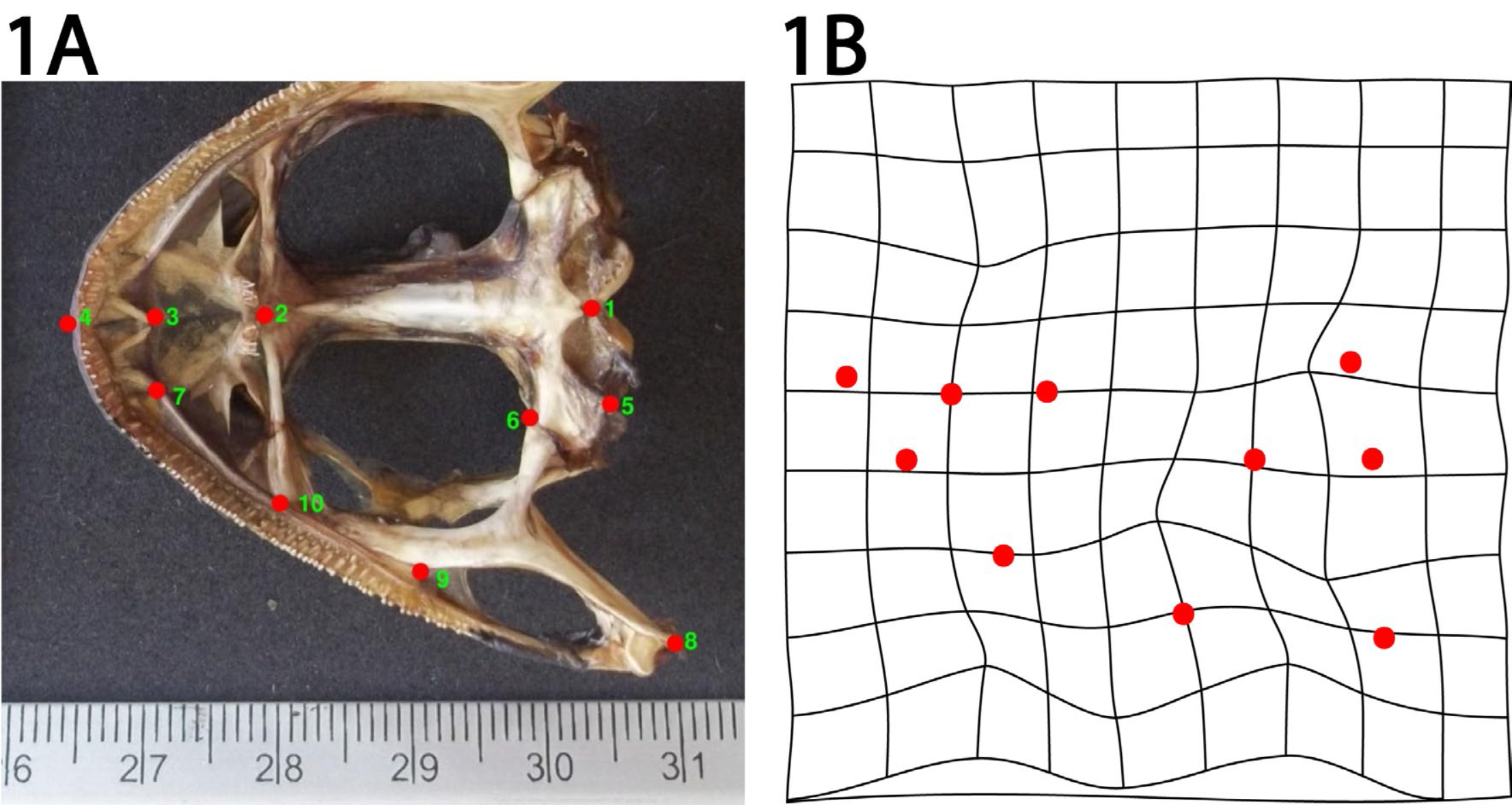
Figure 1 Ventral photograph of a bullfrog skull, showing the ten landmarks used for geometric morphometry. A) Landmark representations are: 1) the medial and dorsal limit of the parasphenoid bone, 2) the midpoint of the vomer bone at the height of the palatine process, 3) the outermost posterior point of the premaxila, 4) the anterior end of the premaxilla at the edge of the skull, 5) the dorso-lateral end of the paraesphenoid bone, 6) the parasphenoid bone and pterygoid plate union, 7) the premaxillary-maxillary suture, 8) the posterior end of the pterygoid-quadratojugal joint, 9) the converging point between the pterygoid plate and the maxilla, and 10) the palatine process of the maxilla. The methods to prepare skulls and process the photographs are detailed in the section “Geometric morphometry”, of the Materials and Methods section. B) Example of a partial warp showing landmark position changes after a Procrustes alignment.
Statistics
Body weight and SVL were used to analyze body condition by means of the SMI value, whereas the statistical correlation between these two variables was estimated with a simple linear regression. A two-way ANOVA was used to assess the effect of locality and sex on body condition variables. Hematological values between groups were compared by one-way ANOVA, followed by the Tukey post-hoc test. Differences were set at p < 0.05.
Multivariate statistics
A principal component analysis was used to study linear morphometry variability. This exploratory method is based on the transformation of a set of possibly correlated variables (like the above mentioned linear measurements), to new uncorrelated variables called principal components (PC, normally more than 3 PCs are obtained in the analysis). By making a correlation matrix including all linear measures, variance of all data can be assessed in a way that allows for each PC to incorporate variation from all linear variables. The first component (PC1) thus integrates the largest proportion of the global variance, followed by the PC2, and so on. In this study, the integration of just two principal components (PC1 and PC2) allowed for a more simple and graphic representation of the total variance (whereas a graphic representation of an 8-dimensional linear data set would be nearly impossible). Moreover, with PCA, the contribution of each individual variable to the overall variance can be estimated, giving valuable information of which phenotypic traits vary the most. A Wilk’s-lambda test was performed to analyze differences in linear morphometry between sexes and localities.
To assess the geometric morphometry of the skull, a canonical discriminant analysis was used. This method has the same principles of the PCA but relies on a covariance matrix for the transformation process of the geometric information (codified in landmarks) into canonical variates (CV). By using this approach, it was possible to calculate the mahalanobis distance between groups, which reflected differences between sexes and betweenlocalities.17,18
To evaluate which linear traits best correlates with hind leg length, a generalized linear model was used. This is a multivariate approach of the ordinary linear regression, which allows for the use of multiple explanatory variables in a linear model that relates to the response variable via a link function. In the present analyses the “identity” link function for the gaussian distribution was chosen, and explanatory variables were selected through a stepwise method (forward stepwise and minimum AIC stopping rule).
Results
The ranges of all studied variables, except for linear corporal measurements, are found in Table 1. The average body weight of juvenile bullfrogs was 296.9 g, differing between localities (p < 0.001) but not between sexes (p = 0.284) (Table 2). Average weight of breeder bullfrogs was 437 g, and it was found to differ both between localities (p < 0.001) and gender (p = 0.009). The mean snout-vent length was 12.6 cm for juvenile individuals, and 14.2 cm for breeder frogs. This variable behaved similarly to weight, in that differences were found between localities (p < 0.001), but not between sexes in juvenile frogs (p = 0.509). Analogous results were obtained for adult breeding frogs with snout-vent length being different between localities (p < 0.001) but not between sexes (p = 0.428). The linear regression of weight on snout-vent length (Fig. 2), showed a high correlation between these two variables in juvenile frogs (r² = 0.66, p < 0.001), whilst a lower coefficient was found for breeder frogs (r² = 0.41, p < 0.001). Finally, the average scaled condition value (SMI) was 304.5 g for juvenile frogs and 446.5 g for breeder frogs. The SMI value was similar between localities (p = 0.279), and between sexes (p = 0.172) in juvenile frogs but differed both between farms (p < 0.001) and gender (p = 0.026) in breeder adults.
Table 1 Biometric and hematologic values of juvenile and breeder bullfrogs.
| Trait | Units | Mean ± SE | CI 95% | Range | |
|---|---|---|---|---|---|
| Juvenile bullfrogs | Weight | g | 296.92 ± 6.03 | 284.8-309 | 180-420 |
| SVL | cm | 12.65 ± 0.6 | 12.49-12.82 | 11.1-13.9 | |
| SMI | g | 304.5 ± 4.3 | 295.9-313.2 | 237-403.6 | |
| PCV | % | 31.05 ± 0.83 | 29.3-32.7 | 17-40.6 | |
| WBC | #/μl | 3710.6 ± 139 | 3430-3990 | 2100-7000 | |
| Neutrophils | #/μl | 1070.6 ± 70 | 928.8-1212 | 189-2184 | |
| % Neut. | 29.33 ± 1.5 | 26.2-32.3 | 09-52 | ||
| Lymphocytes | #/μl | 1949 ± 94 | 1759-2138 | 670-3834 | |
| % Limp. | 52.85 ± 1.4 | 49.9-55.7 | 20-75 | ||
| Monocytes | #/μl | 101.2 ± 21.2 | 58.49-144 | 0-798 | |
| % Mon. | 2.92 ± 0.5 | 1.7-4 | 0-19 | ||
| Basophils | #/μl | 311 ± 31.7 | 248-375.5 | 0-1089 | |
| % Baso. | 8.8 ± 0.7 | 7.3-10.4 | 0-24 | ||
| Eosinophils | #/μl | 191.1 ± 21.7 | 149.3-233 | 0-560 | |
| % Eosi. | 5.4 ± 0.62 | 4.1-6.6 | 0-20 | ||
| Breeder bullfrogs | Weight | g | 437 ± 10.6 | 416.3-458.3 | 196.2-700 |
| SVL | cm | 14.26 ± 0.12 | 14.03-14.5 | 11.21-18.1 | |
| SMI | g | 446.5 ± 10.1 | 426.4-466.5 | 276.3-1006 |
Mean ± standard error, 95% confidence interval (CI 95%), and range of weight, snout to vent length (SVL), scaled mass index (SMI), packed cell volume (PCV), white blood cell count (WBC) and different leukocyte numbers. Units are grams (g), centimeters (cm), percentage in total blood (%) and number of cells per microliter (#/μl). The juvenile bullfrog group included male and female one year-old bullfrogs (n = 60), while the breeder frog group contained three year-old male and female individuals (n = 100).
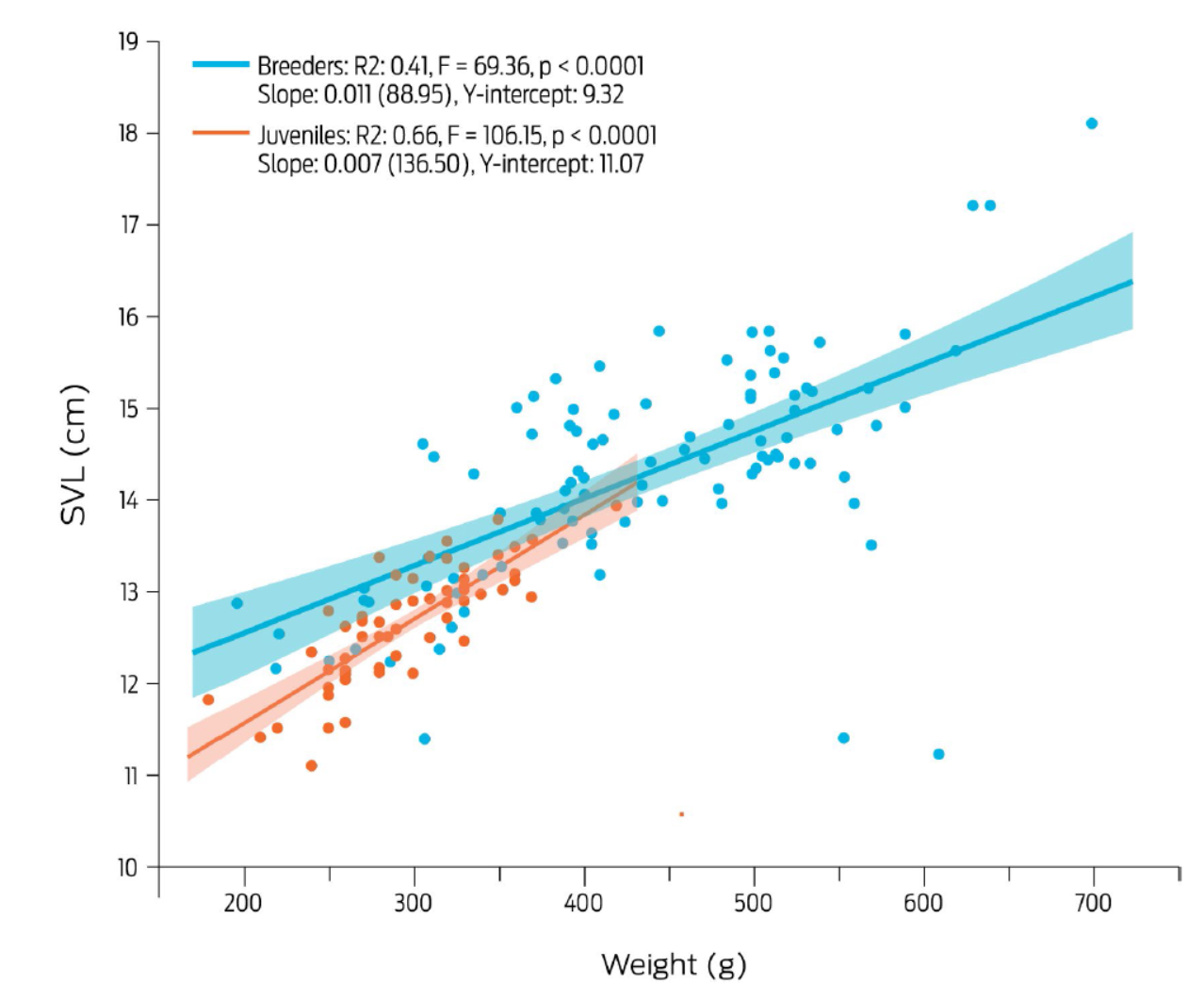
Figure 2 Linear regression of snout to vent length (SVL) and body weight of female and male juvenile bullfrogs (red dots and line, n = 60), and female and male breeder bullfrogs (blue dots and line, n = 100). Dots relate to individual animals, and the lighter colored areas indicate 95% confidence intervals. Correlation coefficients, F-statistics and P values are shown within the figure.
Analyses of hematological values of juvenile bullfrogs showed that the hematocrit was different between localities (p < 0.001), with the lowest values found for animals from the SPT farm. White blood cell count was similar between sexes (p = 0.68) and localities (p = 0.8995). Leukocyte cell type yielded heterogeneous results, with neutrophil being less abundant in specimens collected from the SPT farm, when compared to those that came from the LP site, even when males from the latter location presented the highest values (p < 0.001). No differences were found for lymphocyte number between groups. However, the monocyte count of both males and females in SPT was significantly higher than their LP counterparts (p < 0.001). Moreover, males had a higher monocyte count when compared to females within the SPT location. Finally, basophils and eosinophils were found in equal numbers in all groups of animals.
For breeder females, PC1 and PC2 explained 57.5% and 15.4% of the total variation of linear morphometry, respectively (Fig. 3A). PC1 was dominated by head width and head length, whereas PC2 was dominated by eardrum and eye diameters. For adult males (Fig. 3B), PC1 explained 48.3% of the total morphometric variation, which was mostly affected by snout-vent length and head width values. PC2 on the other hand, explained 13.4% of the phenotypic variation, and was predominantly composed of variation from eye diameter and hind leg size measurements. Linear morphometry was different between sexes (ë = 0.11, p < 0.001) and localities for breeder frogs (Females: ë = 0.04, p < 0.001, Males: ë = 0.06, p < 0.001).
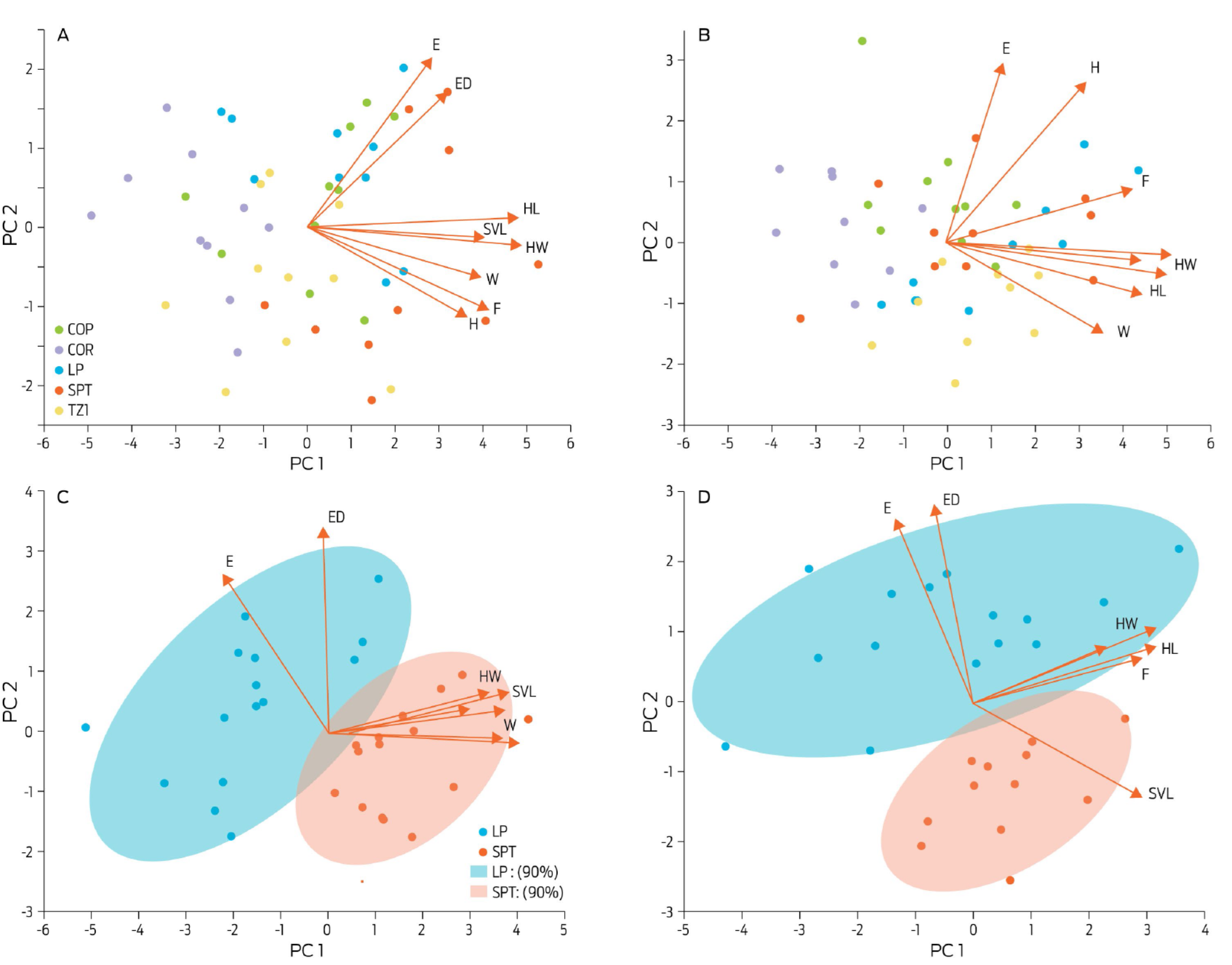
Figure 3 Principal component analysis for the linear morphometry of bullfrogs. This analysis included the eight linear measurements of breeder females (A, n = 50), breeder males (B, n = 50), juvenile females (C, n = 30), and juvenile males (D, n = 30). The principal components 1 and 2 (PC1, PC2) were used as vectors to display each dot as an individual animal. The red arrows relate to the loading vectors of each linear variable. Color ellipses in C and D are the 90% data dispersion intervals. A and B do not have dispersion intervals for a better appreciation of the graph. COP: Copuyo; COR: Villa Corregidora; LP: La Purísima; SPT: San Pedro Tlaltizapan; TZI: Isla de Tizirio.
The variability in linear morphometry was explained by PC1 (55.8%), and PC2 (15.8%) for juvenile females (Fig. 3C). The first component being mainly influenced by snout-vent length, head length, and hind leg size, whereas PC2 was strongly affected by eardrum and eye diameters. In juvenile male bullfrogs (Fig. 3D), PC1 contributed to 42.8% of global variation and was mainly affected by snout-vent length, head length and leg length. As for the female group, most of the variability of the PC2 was due to eardrum length and eye diameter. There were differences for linear morphometry between sexes (ë = 0.13, p < 0.001), and localities (ë = 0.15, p < 0.001 for females, and ë = 0.12, p < 0.001 for males).
Generalized linear models showed that hind leg length variability is influenced mainly by head length (÷² = 28.63, p < 0.001), followed by snout-vent length (÷² = 10.26, p = 0.014) and locality (÷² = 8.02, p = 0.046) in juvenile bullfrogs. For breeder animals, only head length and snout-vent length affected hind leg size (Hind leg size: ÷² = 4.8, p = 0.028; SVL ÷² = 3.88, p = 0.048).
Differences were found for shape of the skull of juvenile frogs (Fig. 4). The mahalanobis distance was different between all groups (p < 0.001). Skull shape displayed sexual dimorphism in individuals from the LP farm (p < 0.001), but not in SPT frogs (p = 0.1). Male skull shape differed between localities (p < 0.001). The anatomical structures that mostly contributed to variation of the skull shape were the medial and dorsal limit of the parasphenoid bone, the dorsolateral end of the parasphenoid bone and the posterior end of the pterygoid-quadratojugal joint, which are located at the skull´s most caudal region (for graphic reference, see Fig. 1).
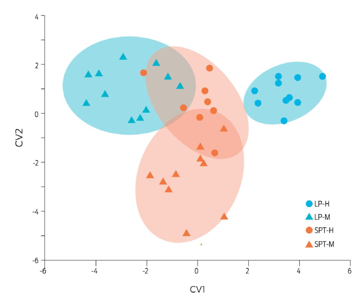
Figure 4 Canonical discriminant analysis for the geometric morphometry of juvenile bullfrog skulls. The CVA analysis included data from juvenile frogs of La Purísima (LP) and San Pedro Tlaltizapan (SPT) localities. LP-females (blue circles, n = 10), LP-males (blue triangles, n = 13), SPT-females (red circles, n = 8), and SPT-males (red triangles, n = 10). Each dot represents an individual, plotted as a vector using the canonical components 1 and 2 (CV1, CV2), of the discriminant analysis. The Procrustes coordinates were taken from 10 landmarks (Fig. 1), determined from ventral photographs of bullfrog skulls. Ellipses correspond to a 90% dispersion interval of data.
Discussion
The size, weight and body condition are relevant phenotypic traits for meat production, since they are directly related to nutritional efficiency.11 Body size and weight values obtained from juvenile and breeding bullfrogs in the present study, were similar to those reported for those obtained in intensive production systems, and for an introduced wild frog population in Brazil.20,21 We observed that breeding females have a higher weight and body condition than males (Table 2) that is probably related to the large egg masses that they produce throughout the year, especially when they inhabit tropical geographic zones.22,23 Gonadal maturation in female bullfrogs begins at one year of age, but do not reach full maturity until year two.24 This could explain the lack of differences in weight and body condition between male and female juvenile bullfrogs. Also, juvenile amphibians use nutrients mainly for body growth, and a redistribution of these resources towards the gonads occur as they mature sexually to favor reproduction.25,26 This could explain why juvenile frogs show a greater correlation between weight and the snout-vent length, when compared with breeder bullfrogs (Fig. 2).
Table 2 Weight, SVL and SMI of juvenile and breeder bullfrogs
| Weight (g) | SVL (cm) | SMI (g) | ||||||||
|---|---|---|---|---|---|---|---|---|---|---|
| Mean | Loc. | Sex | Mean | Loc. | Sex | Mean | bSMA | Loc. | Sex | |
| Juveniles | 296.92 ± 6.03 | < 0.001 | 0.284 | 12.65 ± 0.6 | < 0.001 | 0.509 | 304.5 ± 4.3 | 3.12 [2.6-3.6] | 0.279 | 0.172 |
| Females | 303 ± 8.31 | 12.72 ± 0.11 | 310.4 ± 5.8 | 1.93 [1.2-2.6] | ||||||
| Males | 290.18 ± 8.76 | 12.59 ± 0.12 | 298.1 ± 6.1 | 3.25 [2.6-3.8] | ||||||
| Breeders | 437 ± 10.6 | < 0.001 | 0.009 | 14.26 ± 0.12 | < 0.001 | 0.428 | 446.5 ± 10.1 | 3.03 [2.5-3.5] | < 0.001 | 0.026 |
| Females | 453.44 ± 14.8 | 14.34 ± 0.17 | 466.2 ± 14 | 2.46 [1.8-3] | ||||||
| Males | 421.25 ± 14.8 | 14.19 ± 0.17 | 426.8 ± 14 | 3.88 [3.1-4.6] | ||||||
The mean ± standard error of weight (g), snout to vent length (SVL; cm) and the scaled mass index (SMI; g) (the scaling coefficient bSMA was also included for the analysis) of both juvenile and breeder bullfrogs are shown. The SMI is an adjusted value of weight of each individual, according to a scaling factor bSMA (the slope of a standardized major axis regression of weight on SVL) that is calculated for each group. The p value for the effect of locality and sex is also presented (bold characters indicate significance).
The hematological parameters that were obtained in the present study, give a preliminary reference for bullfrog producers in Mexico (Table 1). Hematocrit and the leukocyte profiles were similar to those reported in previous studies, but lymphocyte number was found to be 10-20% lower.27,28 Consequently, the lymphocyte/neutrophil ratio was also lower. There were differences in the hematocrit and neutrophil count for the LP and STP farms (Table 2), that were probably due to a difference in altitude of approximately 914 meters between the two sites. This has been observed in other anuran species in South America.29
Results of the morphometric analysis showed that there was a high intraspecific variability in American bullfrogs under intensive breeding conditions. In terms of linear morphometry, we found that intraspecific variability in cultured bullfrogs is comparable to that found for Fejervarya limnocharis (Anura, Ranidae) populations, living in Japan, Indonesia and Malaysia,30 where hind leg length and head size contributed a large proportion of the morphometric variability summarized in PC1 and PC2. In terms of geometric morphometrics, the variability of the skull shape in bullfrogs was similar to that found for different morphotypes of the neotropical frog, Proceratophrys cristiceps.15 Therefore, our data suggests the existence of different morphotypes of bullfrogs. However, further studies are needed to clarify whether these groups derive from different genotypes and/or develop as an ontogenetic response to diverse environmental conditions found in bullfrog farms.
Gender was the dominant factor explaining morphometric variability. Given that the bullfrog is a sexually dimorphic amphibian,1,3 this result was expected. As for sources of variability between localities, these could relate to genetic variation, that is common between bullfrog farms since producers exchange breeder frogs frequently to avoid inbreeding (personal communication from several producers). Also, genotype-environment interactions, which affect growth, survival, body morphometry, yield, feeding intake, weight, protein and lipid content, fecundity and skin color should be considered.31 Lastly, developmental plasticity driven by epigenetic regulation in response to environmental factors, which has been reported for species such as Rainbow trout,32,33 Brown trout34 and Atlantic salmon35 could contribute to this variability as well.
Frog legs or haunches are the most high-value commercial product from bullfrog farming.1 However, phenotypic, genetic or environmental variables that may influence their size have not been clearly established. The selection of breeding frogs in Mexico is entirely based on body size and does not consider any other features (personal communication with bullfrog breeders). In the present study we found that the morphometric variable with the greatest correlation with hind leg length is head length, followed by snout-vent length for juvenile and adult breeder frogs, with a weaker association for the latter group. Snout-vent length as a parameter for selection is a common practice in Mexico, however, results from this study show that it is not the best predictor of hind leg size, and thus requires further evaluation. The apparent lack of association between hind leg length and body size, may stem from the fact that appendicular development is decoupled from axial development in anurans, since limb outgrowth begins days or weeks after somites have differentiated.36 Moreover, both leg and head length were the main sources of morphometric variability of PC1, in male and female juvenile individuals (Fig. 3), which means that these are highly plastic variables in bullfrogs, which could be of interest for breeding programs. This is based on the fact that it is during postmetamorphic stages of development that anurans exhibit the greatest amount of morphological variability and also when the skull and whole skeleton become ossified.37
Altogether, the findings in this work suggest that further studies that include genetic (i.e. genetic correlation estimates) and heritability analyses are needed to implement successful breeding programs aimed at enhancing frog leg yield and growth rate of animals.15 Genetic parameters are also needed to design adequate national breeding programs. The effect of factors such as temperature (both in water and air), food quality, population density and diseases on overall body and hind leg growth rates, needs also to be examined.38,39,40,41 We consider that these studies are essential to improving bullfrog production in Mexico. Joint work between academic institutions, producers and government agencies will be essential. Finally, the complete genome of the bullfrog was recently published, which will enable the design of genomic tools that will help improve bullfrog farming and the development of genetically improved strains.42
Conclusions
The present work characterizes phenotypic traits of American bullfrogs under intensive production systems in Mexico. Results provide a start point for the development of appropriate zootechnical management practices that could impact breeding programs for this species at national level. Results from this study show that there is a high phenotypic variability between bullfrog production systems, a fact that could be of use for increasing genetic gains and heterosis rates as has been previously done with fish.43,44,45 Likewise, free-living bullfrog populations could contribute to promote a greater genetic variability in breeding programs.

