


 text new page (beta)
 English (pdf)
 Article in xml format
 Article references
 Send this article by e-mail
 Cited by SciELO
  Similars in
SciELO
Similars in
SciELO 
 Permalink
Introduction
International financial markets, accelerated by the development of technological innovations and the growing competitiveness among its members1, have evolved to become complex markets that influence the development of economies. In this context, FDI is a key element that helps establish stable and lasting links between countries, fostering relations with multilateral benefits.
In general, FDI promotes the transfer of technological innovations that optimize the production and competitiveness of transnational companies (Borensztein et al., 1998; Meltem, 2014). The term FDI refers to business capital that seeks to establish itself locally in other countries and is distinguished from financial investment because it serves as a lever for external financing for companies and industries that seek long-term benefits (Dussel, 2000; Bouchet et al., 2003).
Despite the multiple benefits, each company may be motivated by different characteristics of the host country. In Mexico, the variables that promote efficiency have been especially relevant in recent years (Dussel, 2000; Rivas and Puebla, 2016; Elizalde et al., 2020). According to Rivas and Puebla (2016), efficiency is one of the most important factors because it is related to the country's internal and external productivity and competitiveness.
Among the macroeconomic and microeconomic variables related to the search for efficiency, trade openness, tax levels, the price and quality of labor, technological levels, interest rates, inflation, wage rates, oil prices, among others, stand out. Several authors have incorporated this type of variables to explain FDI in Mexico. Jordaan (2005), using a linear production function, derived from a Cobb-Douglas production function, analyzes FDI and its relationship with external factors in the Mexican manufacturing industry in 1993. His results show that the technological difference encourages trade openness and the competitive benefits it represents. On the other hand, through an analytical VAR model and a VEC (Vector Error Correction) model, Gomes et al. (2013) studied FDI flows in Mexico and Brazil (1990-2010). The results indicate that trade openness, coupled with an autoregressive factor, is the variable with the greatest influence on FDI flows; therefore, it is concluded that the capital invested in Mexico is mainly encouraged by policies that promote trade.
Botello and Dávila (2016) used a Probit Model to explain FDI in Mexico and Chile (2000-2013). According to the authors, the flow of FDI in Mexico is mainly encouraged by skilled labor, cheap labor, natural resources, and fiscal incentives. Likewise, Rivas and Puebla (2016), carried out an empirical analysis of sectoral panel data to learn about the dynamics of FDI in Mexico (2000-2012). The results of the analysis reveal that FDI seeks efficiency in production, and that they are mainly explained by economic growth, labor productivity and international competitiveness. Elizalde et al. (2020) presents an investigation on the macroeconomic determinants of FDI in Mexico (2000-2016). Although they include variables of various criteria, the results of the VAR model indicate that FDI in Mexico is explained by the price of oil and the level of foreign debt, together with an autoregressive factor.
Using an econometric panel data model, Tinoco and Guzmán (2020) point out that the regional variables that determine FDI inflows in Mexico (2000-2018) are labor costs, in total number of companies, regional Gross Domestic Product (GDP) and an autoregressive element of the same investment. Finally, Vega and Armijo (2021) emphasize the importance of foreign trade agreements to boost investment and thus the economy in general. According to the authors, the recently ratified trade agreement between Mexico, the United States and Canada (T-MEC) is favorable for Mexico, however there are measures for the automotive industry2 that will harm internal competitiveness in that sector, thus limiting the export potential. and projecting a decrease in FDI in Mexico by July 2025, five years after its entry into force.
Although these studies incorporate variables related to efficiency to explain investment, no research focuses on analyzing the efficiency variables that stimulate the flow of FDI in Mexico. It is important to deepen the analysis of the variables that promote efficiency because they are related to productivity, competitiveness and distribution networks that the capital invested in Mexico needs.
The main objective of this research is to evaluate the influence of efficiency variables on FDI flows in Mexico in the period 1995-2020. And generate conclusions oriented to the search for actions to attract greater external financing and take advantage of the commercial relations of this country.
Based on preliminary studies, this study posits that macroeconomic efficiency variables, as well as an autoregressive component of FDI itself, determined FDI flows in Mexico for the period 1995-2020. This hypothesis is tested through a VAR model, after applying the Hodrick and Prescott filter for the decomposition of the variables. In the first section, the role played by the efficiency factor in FDI is explained, in the second section the methodology used is described, followed by section three, where the results are disclosed and a discussion is carried out; finally, the fourth section presents the main conclusions.
I. The efficiency factor in fdi
The Economic Commission for Latin America, ECLAC classifies FDI according to the specific purposes that these investments pursue. Multiple investigations3 classify FDI according to criteria such as the search for resources, search for markets, search for efficiency, search for strategic assets and the risk factor.
FDI directed to Mexico, mainly for manufacturing, is in search of regional and global efficiency because it seeks to optimize productivity and form distribution networks that allow lower tariff rates, lower production and distribution costs (Dussel, 2000).
According to García and López (2020), the subsidiaries of multinational corporations that seek to establish themselves in developing countries such as Mexico have advantages over their local competitors because they have more advanced production technologies, labor practices, and marketing processes, which is why they generally have a higher productivity and are better able to bring new products to market. Likewise, they have a geographical diversity in their activities that allows them to have operations and assets in different countries, they can obtain supplies or capital goods from abroad and it is assumed that they have greater access to foreign markets to distribute their products. production. The subsidiaries of multinational corporations focus on efficient productivity and have a greater propensity to import and export than local firms, so they will be looking for markets that allow them to develop in these aspects (García and López, 2020).
In this regard, Alguacil et al., (2002) state that in Mexico there is a link between FDI, economic growth and foreign trade. FDI acts as a force that influences economic growth because it stimulates domestic production, which maintains a positive causal relationship with exports. In other words, economic growth in Mexico and its foreign trade are driven by the export orientation of foreign companies that decide to invest in national territory.
In this sense, the efficiency factor is related precisely to those variables that promote productivity and internal and external competitiveness in investments (Rivas and Puebla, 2016). The formation of distribution networks, low tax rates, training and productivity of human capital, labor and production costs, the degree of commercial openness and international agreements that favor the circulation of goods and people are key in the search for efficiency (Dussel, 2000; Garcia and Lopez, 2020). Therefore, within the macroeconomic variables that promote investment efficiency is the GDP, trade openness, tax rates, interest rates, prices of natural inputs, inflation, costs of cheap and specialized labor, external indebtedness, population growth rate, among others.
GDP is one of the most used variables in empirical studies that seek to explain FDI. In most investigations, this variable is related to the dimensions of the available market; however, Mogrovejo (2005), Jadhav (2012), Tang et al., (2014) and Iamsiraroj (2016) agree that GDP is an indicator of financial development of the host country. In this research, GDP is considered as a variable that promotes efficiency because, according to these authors, a larger financial market represents a greater opportunity for development and profitability. On the other hand, trade openness is represented by the share of foreign trade in GDP; that is, the trade openness index (Bhavan et al., 2011; Jadhav, 2012) and has a positive relationship with FDI flows (Jadhav, 2012; Gomes et al., 2013 and Rivas and Puebla, 2016). In this regard, Rivas and Puebla (2016) state that when exports increase, FDI does too, although to a lesser extent. According to the authors, high levels of exports are related to more competitive and attractive production sectors for new investment capital, while protectionism represents higher transaction costs associated with production costs (Jadhav, 2012). Trade openness also favors the import of capital goods and advanced technologies, which is why it is related to efficiency (Gomes et al., 2013; García and López, 2020).
Among the economic variables that impact the efficiency of invested capital are corporate taxes, these taxes are closely related to the generation of company income; higher tax rates paid by investors affect the profits generated (Meltem, 2014). According to Caballero and López (2012), Meltem (2014) and Tang et al., (2014), taxes maintain an inverse relationship with FDI because they can discourage it, likewise, a low tax rate can improve the competitiveness of the host country. It is important to consider that, in Mexico, those legal entities that are non-residents are obliged to pay taxes when they obtain income from any source of wealth located in Mexican territory (Income Tax and Flat Rate Business Tax). In this regard, Caballero and López (2012) state that in order to stimulate private investment in Mexico, the most appropriate thing is to give investors greater facilities through a controlled Income Tax rate; in México known as ISR.
Another variable to highlight is the interest rate; Schwartz and Torres (2000) mention that the credit channel is the main way of impacting the interest rate because it can affect the capacity for consumption and productive investment. The interest rate is negatively related to FDI through the 28-day TIIE (Meltem, 2014; Varela and Cruz, 2016). An increase in interest rates decreases the demand for credit and with this investment, likewise, if banks consider that investment projects are high risk, they can reduce the credit supply. In this way, the increase in interest rates, coupled with banking uncertainty regarding the quality of investment projects, can lead to a lower availability of credit in the economy (Schwartz and Torres, 2000). In this regard, Varela and Cruz (2016) conclude that multinational corporations not only make capital transfers to invest abroad, but also consider the conditions of the local credit market to make investments in the construction or operation of the plant. Even capital or other goods can be purchased as required by the production process. Given that credit channels can be affected by the evolution of interest rates, their impact on FDI flows is not a minor issue.
Interest rates should make it possible to ease liquidity restrictions, but they should also be a mechanism that avoids serious problems of price instability. To the extent that price stability objectives are met, monetary policy should contribute to achieving more competitive interest rates in the market, so that FDI is favored locally by bank credit channels private (Varela and Cruz, 2016, p. 146).
On the other hand, even though FDI has a direct relationship with the availability of inputs, the price of these maintains an inverse relationship with investment; Oil price increases are related to lower FDI flows. According to Botello and Dávila (2016), low-cost inputs in the host country benefit efficiency by reducing production, transportation, and distribution costs throughout the production chain. A country may be more attractive for investment if, as far as possible, it keeps input costs stable (Jadhav, 2012; Botello and Dávila, 2016).
Likewise, inflation is a determining efficiency variable for FDI because it impacts the purchasing power of consumers, which is related to the demand for goods; inflation maintains an inverse relationship with FDI in the short term (Bittencourt and Domingo, 2002; Bouchet et al., 2003; Mogrovejo, 2005; Madura, 2010). However, a country with low and stable inflationary increases can be attractive, since it reflects macroeconomic stability and the capacity of its government to face expenses and debts in the long term (Cantor and Parcker, 1996; Bittencourt and Domingo, 2002).
On the other hand, even though studies such as Gomes et al., (2013) and Elizalde et al., (2020) catalog cheap labor and skilled labor within the criterion of variables in search of availability of resources, in the present investigation they are considered as variables that promote efficiency, since they are related to the productivity of companies. The resource endowment and trade theory explain that FDI is directed towards countries with low wages and natural resources that provide comparative advantages that contribute to business productivity (Botello and Dávila, 2016). On the other hand, skilled labor can reduce investment uncertainty because it can be seen as an indication of favorable conditions and development in the host country. In areas where there are more skills, there is greater organization, innovation and progress; specialized FDI requires specialized labor for higher productivity (Botello and Dávila, 2016). There is evidence that this variable is important for FDI flows to Mexico4. In recent decades, foreign companies in Mexico have required specialized labor to guarantee labor productivity to achieve productive efficiency and international competitiveness (Rivas and Puebla, 2016).
Finally, it is important to mention that external over-indebtedness is a component of government interference that could affect the profitability or stability of invested capital (Morales and Tuesta, 1998; Dans, 2012). The debt overhang could affect FDI flows in two ways. First, seen as a problem of insolvency in the payment of the debt and classified as an economic risk factor, an increase in over-indebtedness increases the probability of default on financial obligations, which can lead to uncertainty in the future performance of the economy. (Feenstra and Taylor, 2014; Topal and Gül, 2016). Second, seen as a structural problem in which the government aims to meet financial obligations, the profitability of FDI is reduced by the imposition of future taxes, what Krugman (1988) calls the investment tax; this last problem is classified under the criterion of efficiency. In any case, as the debt/GDP ratio increases, the risk of insolvency in the country will be greater (Morales and Tuesta, 1998).
II. Data and estimation procedure
In this research, quarterly time series were used from January 1995 to March 2020. FDI was converted to national currency with the FIX exchange rate5 (Banxico, 2020), and the values were deflated through of the National Consumer Price Index (INPC) base 2018 (INEGI, 2020). The variable GDP is data in millions of pesos (Banxico, 2020); the variable Trade openness (CO) is the share of foreign trade with respect to GDP, that is, CO = (X + M) / GDP where X represents total exports, and M is total imports (Gomes et al., 2013) (Banxico, 2020). The ITR variable is the Income Tax Rate collection with respect to GDP, that is, ITR = TIT / GDP * 100 where TIT represents the Total Income Tax for the period (Caballero and López, 2012) (SHCP, 2020). The OP variable refers to the price of the Mexican oil mix per barrel in dollars (BANXICO, 2021), while INF is the inflation, represented by the National Consumer Price Index with the second half of 2018 as the base (BANXICO, 2021). The IR variable is explained with the reference interest rate in México (28-day TIIE) (Varela and Cruz, 2016) (Banxico, 2021). Finally, it is important to mention that the statistical package used for modeling was SAS version 9.4 (SAS Institute, Inc. 2002-2012).
VAR Model
In the first instance, it seeks to meet the condition of stationarity6 in each variable. Stationary variables, also known as non-integrated variables, are characterized by not having a unit root, this implies that their mean and variance are constant and the covariance between two periods will depend exclusively on the distance between them, which allows predicting with greater ease their behavior (Gujarati and Porter, 2010).
In order to obtain stationary series, the methodology of Hodrick and Prescott (1997) 7 is used to decompose each variable. It is important to mention that this type of filter allows an original series to be decomposed and a new series to be obtained, the magnitude of which is free from any specific effect that hinders the correct interpretation of its values. Subsequently, unit root tests are applied to the variables without trend to confirm whether they comply with stationarity (Quintana and M., 2016).
With the stationary variables, the VAR methodology is implemented. This methodology was developed by Christopher Sims at the beginning of the eighties, who states that in economic theory and mainly in macroeconomics there is not enough knowledge to strictly classify endogenous and exogenous variables. That is, the original intention was to estimate an analytical tool made up of a "dynamic system of variables without using theoretical perspectives" (Sims, 1980, Gujarati and Porter, 2010 and Quintana et al., 2016).
It is a simultaneous equations model formed by a reduced unrestricted system of equations, whose purpose is to characterize the interactions between a group of variables and identify the effects of any variable on another in the model. The variables can be correlated contemporaneously but not through different periods, in addition, none of the coefficients is assumed to be zero a priori and the specification is unrestricted in that all the variables have the same number of lags "p" (order of the VAR model) (Gujarati and Porter, 2010 and Quintana et al., 2016).
It should be noted that in these models the degrees of freedom are restricted, so twenty combinations of three efficiency variables were made to explain the investment. Equation 1 represents the linear relationship between FDI and the first combination of variables (GDP, CO and ITR). It is important to mention that all the variables are represented at time "t" and the sign represents the expected relationship:
Where the terms 𝛼´s represent the coefficients of the variables (GDP CO ITR), “𝑐” symbolizes the intercept and ε is an error term at time “t”. It is worth mentioning that this equation represents only the long-term equilibrium relationship between the variables.
On the other hand, the general formulation of the VAR model with the first combination of explanatory variables is defined as follows:
Where on the left side we have the vector (4x1) made up of the variables of the system of equations in period t. On the right side is the vector of constant terms α of (4x1), to which is added the matrix of autoregressive coefficients β of (4x11) multiplied by that of lagged variables from t-1 to t-p of (4x1). Finally, the vector of errors ε (innovations or impulses) in period t.
The order of the VAR model is defined according to the Akaike Information Criterion (AIC). Once the order of the model has been defined, the causality of the variables is verified through the Engle-Granger causality test. It is important to carry out this test because in regression analysis the dependence of one variable on others does not necessarily indicate the existence of causality.
Subsequently, statistically significant variables and lags are located in the FDI equation through their calculated t-statistic. Continuing with the example of the first combination of explanatory variables, the independent FDI equation is theoretically expressed as follows:
FDI at time “t” is explained by its constant term α, to which is added the matrix of autoregressive coefficients β of (1x4) multiplied by that of lagged variables from t-1 to tp of (4x1) plus the error term ε (innovation or impulse) in period t.
In the last stage, the model that best adjusts to FDI is identified through the AIC criterion and the absolute mean percentage error (MAPE), the latter is a percentage statistical indicator that allows measuring the accuracy of the model prediction. Likewise, by way of diagnosis, a simple regression of the predicted data is carried out against the observed data, the resulting adjusted R-squared also allows the accuracy of the prediction to be measured. Finally, in order to identify the average impact of each variable in monetary terms, simulations are carried out in the Excel program.
III. Results and discussion
Using the Hodrick and Prescott (1997) methodology, each variable is broken down and the trend component is subtracted. Next, the results of the decomposition models are presented (Table 1) and the graphs represent the trend, irregular and cyclical components of the variables.
Table 1 Descomposición models
| Variable | AIC | Ajusted-R2 |
|---|---|---|
| FDI | 120.80 | 0.63016 |
| GDP | -435.80 | 0.97293 |
| CO | -284.90 | 0.99088 |
| ITR | -90.09 | 0.95257 |
| OP | -34.32 | 0.9122 |
| INF | -560.80 | 0.9984 |
| IR | -100.50 | 0.9545 |
Source: Author’s elaboration
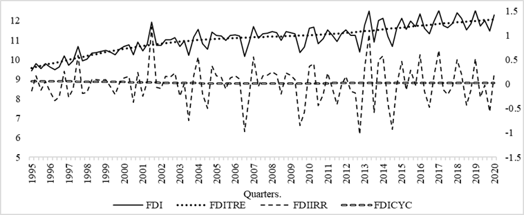
Note: FDI (Foreign Direct Investment), FDITRE (Trend), FDIIRR (Irregular), FDICYC (Cyclical).
Source: Author’s elaboration
Figure 1 FDI and its components.
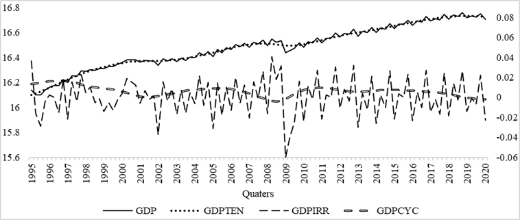
Note: GDP (Gross Domestic Product), GDPTRE (Trend), GDPIRR (Irregular), GDPCYC (Cyclical).
Source: Author’s elaboration
Figure 2 GDP and its components
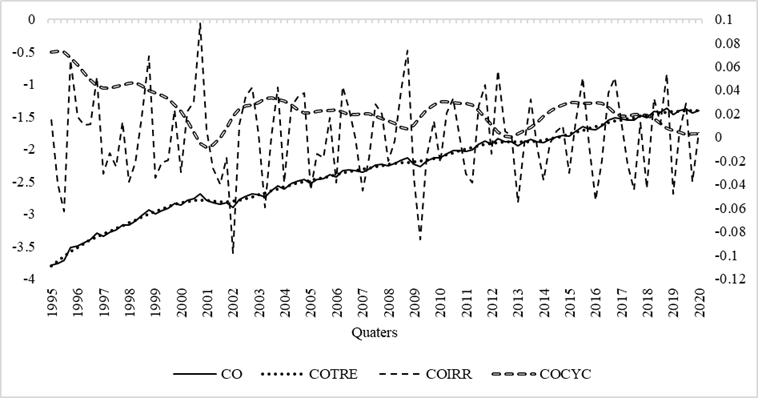
Note: CO (Trade openness), COTRE (Trend), COIRR (Irregular), COCYC (Cyclical).
Source: Author’s elaboration
Figure 3 CO and its components
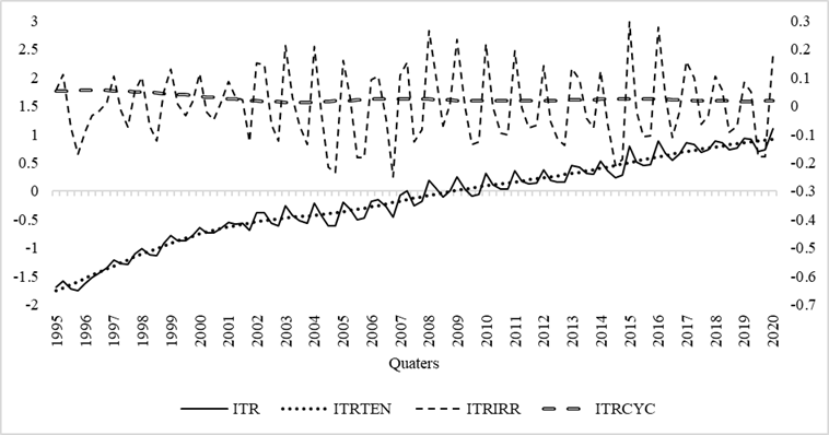
Note: ITR (Income Tax Rate), ITRTRE (Trend), ITRIRR (Irregular), ITRCYC (Cyclical).
Source: Author’s elaboration
Figure 4 ITR and its components
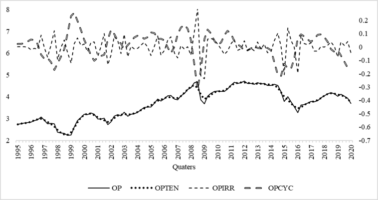
Note: OP (Price of the Mexican oil mix), OPTRE (Trend), OPIRR (Irregular), OPCYC (Cyclical).
Source: Author’s elaboration
Figure 5 OP and its components
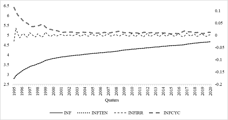
Note: INF (Inflation), INFTRE (Trend), INFIRR (Irregular), INFCYC (Cyclical).
Source: Author’s elaboration
Figure 6 INF and its components.
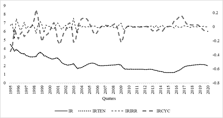
Note: IR (Interest rate), IRTRE (Trend), IRIRR (Irregular), IRCYC (Cyclical).
Source: Author’s elaboration
Figure 7 IR and its components
Subsequently, through the Augmented Dickey Fuller and Phillips Perron unit root tests, it is verified whether the variables without trend (FDI2, GDP2, CO2, ITR2, OP2, INF2 and IR2) present a stationary behavior (Table 2).
Table 2 Unit root tests
| Variable | DFA | PP |
|---|---|---|
| Prob<F in tiers | Prob<T in tiers | |
| FDI2 | < 0.0001 | < 0.0001 |
| GDP2 | < 0.0001 | < 0.0001 |
| CO2 | < 0.0001 | < 0.0001 |
| ITR2 | < 0.0001 | < 0.0001 |
| OP2 | < 0.0001 | < 0.0001 |
| INF2 | < 0.0001 | < 0.0001 |
| IR2 | < 0.0001 | < 0.0001 |
Ho: Exist unit root.
Source: Author’s elaboration
The results indicate that at a significance level of 5%, the existence of a unit root is rejected for all variables; therefore they are integrated variables of order zero I(0).
According to the statistical evidence, the VAR model made up of the variables FDI2, CO2, ITR2 and IR2 is the one that best fits. The AIC information criterion of the lag exclusion test indicates that the optimal lag is six (Table 3).
Table 3 Lag exclusion test
| VAR | AICC | HQC | AIC | SBC | FPEC |
|---|---|---|---|---|---|
| 1 | -20.2006 | -20.0452 | -20.2139 | -19.7971 | 1.66E-09 |
| 2 | -20.866 | -20.5834 | -20.9228 | -20.084 | 8.20E-10 |
| 3 | -21.2784 | -20.903 | -21.4151 | -20.149 | 5.03E-10 |
| 4 | -21.6505* | -21.2243 | -21.9112 | -20.2124* | 3.09E-10 |
| 5 | -21.6194 | -21.1942 | -22.058 | -19.921 | 2.70E-10 |
| *6 | -21.6355 | -21.2759* | -22.3187* | -19.7379 | 2.12E-10 |
| 7 | -21.2194 | -21.0064 | -22.2304 | -19.2001 | 2.39E-10 |
*Optimal lag according to each criterion
Source: Author’s elaboration
After establishing the optimal number of VAR lags, the Engle Granger causality test is performed. As can be seen in Table 4, test 1 indicates that the variables CO2, ITR2 and IR2 cause FDI2 in the Granger sense to a significance level of 5% in lag six.
Table 4 Engle Granger causality test
| Test | Lags | Tipe | Estadistic | Pr > ChiSq | Contrast |
|---|---|---|---|---|---|
| Test 1 | 6 | Wald | 57.67 | <.0001 | CO2, ITR2, IR2 → FDI2 |
| Test 2 | 6 | Wald | 54.14 | <.0001 | FDI2, ITR2, IR2 → CO2 |
| Test 3 | 6 | Wald | 33.48 | 0.0146 | CO2, FDI2, IR2 → ITR2 |
| Test 4 | 6 | Wald | 73.65 | <.0001 | CO2, ITR2, FDI2 → IR2 |
Source: Author’s elaboration
The results of the VAR (6) model indicate an adjusted R squared of 0.3616 and an AIC of -22.3187. Next, the parameters of the VAR (6) for the FDI2 variable are presented (Table 5).
Table 5 FDI2 VAR (6) Parameters
| Parameter | Estimate | Standard Error | t Value | Pr > |t| | Variable |
|---|---|---|---|---|---|
| AR1_1_1 | -0.2543 | 0.10875 | -2.34 | 0.0222 | FDI2(t-1) |
| AR1_1_2 | -0.88542 | 1.35986 | -0.65 | 0.5171 | CO2(t-1) |
| AR1_1_3 | 1.16027 | 0.56279 | 2.06 | 0.0429 | ITR2(t-1) |
| AR1_1_4 | -0.64289 | 1.93209 | -0.33 | 0.7403 | IR2(t-1) |
| AR2_1_1 | -0.37262 | 0.10879 | -3.43 | 0.001 | FDI2(t-2) |
| AR2_1_2 | -0.08674 | 1.37204 | -0.06 | 0.9498 | CO2(t-2) |
| AR2_1_3 | 1.01401 | 0.53896 | 1.88 | 0.064 | ITR2(t-2) |
| AR2_1_4 | -4.15316 | 2.32461 | -1.79 | 0.0783 | IR2(t-2) |
| AR3_1_1 | 0.00044 | 0.12112 | 0 | 0.9971 | FDI2(t-3) |
| AR3_1_2 | 1.36061 | 1.36425 | 1 | 0.322 | CO2(t-3) |
| AR3_1_3 | -0.01399 | 0.45044 | -0.03 | 0.9753 | ITR2(t-3) |
| AR3_1_4 | -4.96693 | 2.78557 | -1.78 | 0.0788 | IR2(t-3) |
| AR4_1_1 | -0.09248 | 0.12332 | -0.75 | 0.4558 | FDI2(t-4) |
| AR4_1_2 | -1.8241 | 1.39289 | -1.31 | 0.1946 | CO2(t-4) |
| AR4_1_3 | 0.16145 | 0.44615 | 0.36 | 0.7185 | ITR2(t-4) |
| AR4_1_4 | -5.83239 | 2.6409 | -2.21 | 0.0304 | IR2(t-4) |
| AR5_1_1 | 0.00858 | 0.11694 | 0.07 | 0.9417 | FDI2(t-5) |
| AR5_1_2 | 2.02062 | 1.52015 | 1.33 | 0.188 | CO2(t-5) |
| AR5_1_3 | -0.88334 | 0.51738 | -1.71 | 0.0921 | ITR2(t-5) |
| AR5_1_4 | -8.27618 | 2.26286 | -3.66 | 0.0005 | IR2(t-5) |
| AR6_1_1 | -0.02123 | 0.11697 | -0.18 | 0.8565 | FDI2(t-6) |
| AR6_1_2 | 5.65457 | 1.60056 | 3.53 | 0.0007 | CO2(t-6) |
| AR6_1_3 | -1.10097 | 0.52654 | -2.09 | 0.0401 | ITR2(t-6) |
| AR6_1_4 | -5.27623 | 1.72396 | -3.06 | 0.0031 | IR2(t-6) |
Source: Author’s elaboration
As can be seen in Table 5, most of the parameters are not statistically significant for the FDI2 variable, therefore, the model is improved by discarding the non-significant parameters through the t-test with a significance level of 10%. (Table 6). As a result, a model for FDI2 with a best adjusted R squared of 0.4142 is obtained:
Table 6 Fitted model parameters FDI2
| Parameter | Estimate | Approx Sth Err | t Value | Approx Pr > |t| |
|---|---|---|---|---|
| A1 | -0.23791 | 0.0886 | -2.68 | 0.0088 |
| A3 | 1.167704 | 0.4711 | 2.48 | 0.0153 |
| A5 | -0.34848 | 0.0878 | -3.97 | 0.0002 |
| A7 | 0.942447 | 0.4393 | 2.15 | 0.0349 |
| A8 | -3.17106 | 1.4519 | -2.18 | 0.0319 |
| A11 | -0.24974 | 0.3288 | -0.76 | 0.4497 |
| A12 | -3.47677 | 1.6257 | -2.14 | 0.0355 |
| A14 | -1.73006 | 0.9979 | -1.73 | 0.0868 |
| A16 | -5.15277 | 1.8803 | -2.74 | 0.0076 |
| A18 | 2.214266 | 1.1889 | 1.86 | 0.0662 |
| A19 | -0.78221 | 0.4076 | -1.92 | 0.0585 |
| A20 | -7.76068 | 1.7931 | -4.33 | <.0001 |
| A22 | 5.131248 | 1.2007 | 4.27 | <.0001 |
| A23 | -1.17413 | 0.4020 | -2.92 | 0.0045 |
| A24 | -4.78638 | 1.3919 | -3.44 | 0.0009 |
Source: Author’s elaboration
Subsequently, the estimated values of FDI2 are printed and the trend is added to obtain the estimated FDI (FDIf). Figure 8 shows the observed FDI and estimated (FDIf).
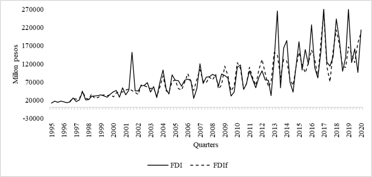
According to this adjusted model (Equation 2), the FDI2 in time “t” is inversely related to its previous first and second quarters; likewise, there is an inverse relationship with the lagged fourth quarter of Co2, but positive with the fifth and sixth quarters. On the other hand, the model suggests that there is a positive relationship with the first two lagged quarters of ITR2, but an inverse relationship with its third, fifth and sixth lags. Finally, an inverse relationship can be observed with the second, third, fourth, fifth and sixth lagged quarters of IR2.
As mentioned above, this VAR methodology is applied for each of the twenty combinations of variables. Table 7 presents the optimal lag of each model according to the AIC criterion, as well as the mean absolute percentage error (MAPE) and the adjusted R-squared of each combination.
Table 7 VAR Models
| Combination | Optimal lag | AIC | MAPE | Adj-R2 | |
|---|---|---|---|---|---|
| 1 | FDI2, GDP2, CO2, ITR2 | 6 | -23.1724 | 22.9759 | 0.3646 |
| 2 | FDI2, GDP2, CO2, OP2 | 6 | -24.3279 | 22.4921 | 0.3834 |
| 3 | FDI2, GDP2, CO2, INF2 | 6 | -30.5444 | 23.5534 | 0.3580 |
| 4 | FDI2, GDP2 CO2, IR2 | 6 | -25.9696 | 22.6441 | 0.3849 |
| 5 | FDI2, GDP2, ITR2, OP2 | 6 | -22.1526 | 22.3487 | 0.3956 |
| 6 | FDI2, GDP2, ITR2, INF2 | 6 | -28.2819 | 24.2088 | 0.3294 |
| 7 | FDI2, GDP2, ITR2, IR2 | 6 | -23.8619 | 24.9859 | 0.3040 |
| 8 | FDI2, GDP2, OP2, INF2 | 6 | -29.2567 | 24.8307 | 0.2348 |
| 9 | FDI2, GDP2, OP2, IR2 | 6 | -24.7623 | 24.7801 | 0.2208 |
| 10 | FDI2, GDP2, INF2, IR2 | 6 | -310425 | 24.0869 | 0.2411 |
| 11 | FDI2, CO2, ITR2, OP2 | 6 | -19.9174 | 22.0884 | 0.3970 |
| 12 | FDI2, CO2, ITR2, INF2 | 6 | -26.5629 | 23.8529 | 0.3342 |
| *13 | FDI2, CO2, ITR2, IR2 | 6 | -22.3187 | 20.5978 | 0.4142 |
| 14 | FDI2, CO2, OP2, INF2 | 6 | -27.2160 | 25.8303 | 0.2258 |
| 15 | FDI2, CO2, OP2, IR2 | 6 | -22.0039 | 21.1440 | 0.4138 |
| 16 | FDI2, CO2, INF2, IR2 | 6 | -29.3587 | 25.0514 | 0.2370 |
| 17 | FDI2, ITR2, OP2, INF2 | 6 | -25.1388 | 23.2788 | 0.3455 |
| 18 | FDI2, ITR2, OP2, IR2 | 6 | -20.5827 | 23.3388 | 0.3702 |
| 19 | FDI2, ITR2, INF2, IR2 | 6 | -27.3035 | 25.1417 | 0.2546 |
| 20 | FDI2, OP2, INF2, IR2 | 6 | -27.6072 | 25.5597 | 0.2317 |
*Best combination
Source: Author’s elaboration
It is important to mention that the selected model presented a MAPE of 20.6%, this indicates that it predicts the behavior of FDI by 79.4%. Likewise, as a diagnosis, a regression is performed between FDI and the predicted values (FDIf), the result of which is an adjusted R-squared of 0.7714.
To capture the impact of efficiency variables on FDI, simulations are carried out in the period 1995-2020. The results indicate that a 10% increase in the lagging quarters of FDI2 generates an average decrease of 2.87% in FDI, which represents a drop of 2,473.8 million pesos. On the other hand, a 10% increase in the lagging quarters of CO2 generates an average increase 0.47% in FDI, which represents an increase of 347.7 million pesos. Likewise, a 10% increase in the lagging quarters of ITR2 generates an average decrease of 0.09% in FDI, which represents a drop of 3.0 million pesos. Finally, a 10% increase in the lagging quarters of IR2 generates an average decrease of 3.80% in FDI, which represents a drop of 2,229.8 million pesos. This relationship between variables reveals the sensitivity of FDI in Mexico to changes in efficiency variables.
IV. Analysis and discussion
According to the results, the interest rate is the efficiency variable with the greatest impact on external productive investment; there is a significant inverse relationship in the period 1995-2020. However, it is important to take into account that, in recent years, the central objective of monetary policy has been inflationary stability, on many occasions, at the expense of less competitive interest rates in the market8. In this regard, León and De la Rosa (2005) agree that monetary policy has managed to control prices in the markets but has not been aimed at favoring private investment locally through bank credit channels. The interest rate impacts credit availability and with it the consumption capacity of the market and investment; therefore, to the extent that inflationary stability allows it, a monetary policy aimed at achieving competitive interest rates would allow greater access to credit, which would benefit consumption and would be an alternative for investors seeking internal financing for construction. acquisition of inputs, and any other activity related to production processes.
The second variable with the greatest impact is the lagged values of FDI itself. It is worth mentioning that this result coincides with other research9, and indicates that FDI evolves based on its past dynamics due to an adaptive expectation in the short term, or what can be called the reinforcement effect of past flows (Tinoco and Guzmán, 2020). In any case, this result suggests that Multinational Companies make their investment or reinvestment decisions in Mexico considering the dynamics of historical investment flows.
Third, trade openness is a determining variable for attracting FDI in Mexico. The significant positive relationship indicates that greater openness stimulates investment, which suggests that the process of commercial opening initiated in the 1990s, the promotion of trade, the reduction of import tariffs and the ratification of international treaties have benefited the flow of investments10. Various investigations11 agree that greater imports favor the flow of capital goods and technologies that improve transaction costs associated with production costs. Likewise, higher exports are related to more attractive productive sectors for foreign capital because access to international markets favors competitiveness. Therefore, a foreign policy aimed not only at ratifying agreements, but also at reaching agreements that promote a beneficial trade opening for Mexico will be essential.
Finally, Income tax rate is the variable with the least influence on FDI; its significant inverse relationship indicates that high taxes discourage investment due to its close relationship with the profitability of companies. The foregoing suggests that Mexico's tax policy in recent years, focused on maintaining relative stability in income taxes, has benefited the flow of investments12. Moderate Income Tax rates represent lower costs in the start-up or operation of investment projects. Likewise, research such as Caballero and López (2012) emphasize the importance of good administration of the resources captured by taxation. According to the authors, public spending oriented towards economic reactivation and expansion, resulting from good resource management, allows better economic benefits because private investment will be stimulated by the infrastructure provided by the State, and by the additional demand resulting from government spending. Therefore, a tax policy aimed at attracting investment through moderate Income tax rates and good management of tax revenues could generate certainty in investors and, in turn, would be contributing to sustained and stable growth rates.
Conclusions
The hypothesis that macroeconomic efficiency variables and an autoregressive component of FDI itself determined FDI flows in Mexico in the period 1995-2020 is confirmed; however, not all the efficiency variables considered at first were statistically significant.
Likewise, this analysis makes it possible to specify that the implementation of measures in monetary policy, foreign trade and tax policy can be alternatives to favor FDI in Mexico. In the first place, if this country seeks to be more attractive for investment, it should consider, to the extent that inflationary stability allows it, a monetary policy aimed at achieving interest rates that allow greater access to credit, which would benefit the consumption capacity. and they would be an alternative for investors seeking internal financing for their production processes. In the second place, a foreign policy aimed not only at ratifying agreements, but also at achieving agreements that promote a beneficial commercial opening for Mexico will be essential. And finally, a tax policy aimed at attracting investment through moderate income tax rates and good management of tax revenues could improve the profitability and productivity of companies.
These policies are focused on promoting efficiency in FDI because they are closely related to productivity, competitiveness, and distribution networks that capital invested in Mexico needs. Additionally, it is important to mention that these measures can generate the environment of certainty that investors are looking for in a health emergency situation such as the one we are facing. Finally, it is recommended to use the approach of this document in future research; analyzing the efficiency variables in the flow of FDI from other economies or regions can help complement or contrast the results and contribute to the empirical evidence.

