


 text new page (beta)
 English (pdf)
 Article in xml format
 Article references
 Send this article by e-mail
 Cited by SciELO
  Similars in
SciELO
Similars in
SciELO 
 Permalink
Introduction
The economic growth of Mexico has been poor in the past four decades. And, although the economy has been stabilized in terms of inflation and debt, we have not seen again the high growth rates that Mexico had during the 60’s and 70’s. Likewise, despite the many structural reforms implemented at the end of the twentieth century, and more recently in 2013, the Mexican GDP has not grown as it was expected, in part due to the unfavorable external conditions. In this context a natural question is, how a developing economy, such as Mexico, could increase its growth rates?
In this paper, I propose to look at the education as a factor that promotes the economic growth in the long run and, which I consider a main component of human capital. Indeed, recently Manuelli et al. (2014) showed that human capital could be a more important factor of economic growth than what other authors have thought (Klenow et al. [1997]; Hall et al. [1999]; Parente et al. [2000]; and Bils et al. [2000]), and whom, in fact, downplayed the role of human capital in explaining economic growth. Specifically, the model proposed by Manuelli et al. (2014), implies that a large fraction of the cross-country differences in output are due to differences in the quality of human capital.
Likewise, other authors (Pelinescu [2015] and Teixeira et al. [2016]) have found empirical results that are consistent with the economic theory. Human capital improves the quality of labor, increasing its productivity and, hence, the economic growth. Hence, they have found a significant relationship between GDP per capita and human capital.
Nonetheless, we could say that the debate about the importance of human capital on the economic growth is still open. Indeed, some authors have suggested that human capital could be negatively related to employment rates (Ramos et al. [2009] and Čadil et al. [2014]). This negative relationship between employment and human capital (measured as educational attainment) can be observed in Mexican data (see Figure 1).
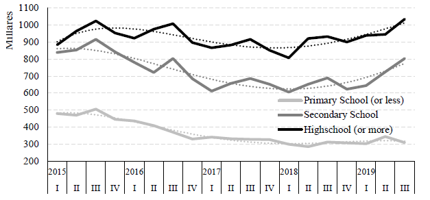
Source: Own elaboration with data of ENOE survey, INEGI.
Figure 1 Number of unemployed Mexican workers
We observe that, for Mexican data, the unemployment rate has an inverted U shape with respect to school attainment. This means that unemployment increases with schooling until college education, but those agents with graduate education levels have a lower unemployment rate (see Table 1, Figure 2). However, this negative correlation does not necessarily imply that human capital induces less growth. It could be the case that the positive effect of schooling can only be realized after an economy crosses a threshold level of development (Ahsan et al., 2017), which have not been reached yet by the Mexican economy.
Table 1 Unemployment for years of schooling
| Schooling | Unemployment rate | |
| Primary School (<6 years) | 2.06 | |
| Secondary School (6-9 years) | 3.75 | |
| Highschool (9-12 years) | 4.54 | |
| College (12-16 years) | 5.55 | |
| Master (16-18 years) | 4.31 | |
| PhD (>18 years) | 1.49 |
Source: ENOE 2019-III, INEGI.
On the other hand, with respect to the role of education, Hanushek et al. (2008) find that there is strong evidence that cognitive skills of population are powerfully related to individual earnings and economic growth. This is because education increases human capital of labor force, which increases labor productivity and transitional growth toward a higher equilibrium output level. But also, because education increases the innovative capacity of the economy, knowledge of new technologies, products and processes, and thus promotes growth (Benos et al., 2014).
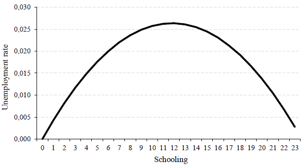
Note: Fitted values from a quadratic regression of unemployment on schooling.
Source: Own elaboration.
Figure 2 Mexican unemployment rate by schooling
It is important to mention that there are two issues that are not addressed in this paper, but which are interesting for future research on the role of human capital in developing economies, for Mexico. The first one is the quality of education. Despite the gap between developed and developing economies has been partially reduced in terms of school attainment, there is still a serious gap in terms of the quality of education, which could play an important role for explaining the effect of education on economic growth (Hanushek, 2013).
The second issue is the labor market segmentation. Recently, it has been noticed the importance of considering a duality of forces in the labor market of developing countries (Alcaraz et al. [2015] , Valdivia et al. [2011] and Maloney [2004]). Indeed, in Mexico, two types of workers coexist in the labor market; those who belong to the formal sector and those who work in the informal sector. The crucial aspect of this duality is that a reduction of the fraction of workers in the informal sector could potentially increase productivity and, hence, increase economic growth.
Although the quality of education and the labor market segmentation are determinant factors, in this research I only focus on the education (measured as years of schooling) of a representative agent, as a variable that drives the economic growth of Mexico. I draw on the Uzawa-Lucas model (ULM), by using time series of the last thirteen years (on a quarterly basis). The reason why I use the ULM among the other endogenous growth models, which represent the household behavior, is because the former has a simpler and realistic representation of an economy, considering human capital as a core element. Thus, the ULM let me measure the role of human capital in the economy of a two-sector dynamic model. Since the sector that produces human capital is well defined in the model, I just had to introduce the role of education in the human capital accumulation. That is why I propose a VEC model of human capital, where schooling is one of the elements of it.
The estimation and interpretation of the model coefficients let me conclude that a one-percent increase in the human capital growth rate, in the long run, produces an increase of 1.59 percent in the Mexican GDP growth. Likewise, an increase of one percent in schooling causes an increase in long run GDP growth rate of 2.19 percent.
The remaining of the paper is organized as follows: In the first section I discuss the state of the art. In the second section I describe the theoretical economic growth model of Uzawa-Lucas. I present the empirics in the third section and explain the data and the Generalized Method of Moments (GMM). The results are presented in the fourth section and finally, the conclusions are presented.
I.Literature Review
One of the first papers that studied the effect of education on the economic growth of Mexico was conducted by Fuller et al. (1986), who find that improvements in the quality of education are more important than the expansion of education itself. Since then, the quality of education in Mexico has reached a minimum required level, so we expect to find a positive effect of education on economic growth even though the quality of education remains the same.
After the seminal contributions of Fuller et al. (1986), Díaz-Bautista (2000) highlights the role of human capital on the regional convergence among the states of Mexico and on the economic growth. Similar results are exposed by García-Verdú (2007), who finds that increases in educational attainment account for nearly one third of real GDP per worker.
The most related paper with my research is the one conducted by Gong et al. (2004), who modify the effects of education and human capital on growth in their variant of Uzawa-Lucas growth model, and test it using time series data from United States (U.S.) and Germany for the period 1962-I to 1996-IV. Gong et al. (2004) consider two versions of the model. The first version assumes that the time spent on education is exogenous and given and does not consider the external effect of human capital. In the second version, the time spent on education is an endogenous variable and the external effect of human capital is considered. Their results show that the model is consistent with the time series of U.S. and Germany, and that there is a nonlinear relationship between human capital and economic growth in both economies.
However, Gong et al. (2004) obtained a negative rate of accumulation of human capital in the original version of the ULM, which makes no sense. That is why they propose a modified version of the model.
From my knowledge, there are no other studies that examine the role of education in the economic growth of Mexico using endogenous growth models, however, there are some studies that get results pointing out to the positive effects of education on economic growth. For example, Ocegueda et al. (2004) analyze the process of regional growth in the border states of Mexico and the U.S. during the period 1975-2000. Their results suggest that human capital and economic specialization have played an important role in economic growth.
Additionally, related literature yields results that are consistent with theoretical predictions, despite its arguably rigurosity, for instance, Ocegueda et al. (2013) use panel data with human capital as the proportion of the population with some level of training obtained in different grades. The authors find that education played an important role in stimulating Mexican economic growth in the period 1990-2008. In another study, Meza et al. (2012) analyze whether the curse of natural resources is present in Mexico. For that purpose, they examine education and human capital during the period 1993-2003 and show that indeed natural resources affect economic growth negatively, while a greater level of education contributes positively. Nevertheless, caution should be taken with their results since they do not correct for endogeneity problems in their models.
On the other hand, Caselli et al. (2013) seek to answer the question of how GDP per worker would increase if workers had more schooling. To do this, they use an approximation to the problem by means of a nonparametric upper bound on output growth generated by more schooling. Their results suggest that, in 2000, if Mexican schooling increased at U.S. level (from 9 to 13 years of schooling), the Mexican GDP would increase by up to 88.6 percent. For the whole sample of 90 countries GDP growth would increase 61 percent, on average.
Interestingly, Hanushek et al. (2012) studied a puzzle among Latin American economies about the fact that the school attainment has increased but not the economic growth, in that region. The authors suggest that we should study the educational achievement, which fully accounts for the poor growth performance of Latin American countries. Nonetheless, for the case of Mexico, Levy and López-Calva (2016) explain the puzzle using the school attainment, they claim that highly educated workers are misallocated in firms that are intense in low educated workers.
In this research paper, I include the education measured as years of schooling (educational attainment), which means that the estimated effect of education on economic growth could be greater if we also increase the quality of education. I base my estimations on the ULM, and I estimate the parameters of technology and preferences with Mexico's time series data using the GMM. I also propose a VEC model in order to consider the role of education on human capital. This helps me to answer whether education has a positive effect on economic growth rates of Mexico.
II.The Uzawa-Lucas Model
The Uzawa-Lucas Model (ULM) is an endogenous growth model since the savings rate is endogenously determined by the parameters of preferences and technology. It contains scale effects in the sense that the increase in human capital formation increases the rate of balanced growth. The model has two sectors, one that produces the physical good using labor, physical capital and human capital, while the other produces the human capital using only human capital. The physical good can be consumed or invested in the creation of physical capital goods. The agent's preferences over consumption streams are defined as:
where L is labor, p is the discount factor,
I assume that in the economy there is a representative skilled worker with ability level h, who spend a fraction u(t) of her no-leisure time to the current production, while she spends a fraction (1-u(t)) of her no-leisure time to the accumulation of human capital.
The resources constraint is given by:
where
The equation (2) implies that human capital is a non-excludable public good but is a rival one.1 Lucas (1988) uses the following linear formulation of Uzawa-Rosen:
where κ is the maximum growth rate of human capital.
The intuition of equation (3) is as follows: if no effort is devoted to human capital
accumulation,
In summary, the solution of the model is given by the following maximization problem over consumption and the proportion of no-leisure time spent in the production sector:
subject to the resource constraint and the Uzawa-Rosen condition for human capital accumulation:
According to Lucas (1988), in the presence of
an external effect
An optimal path is defined as the choice of K(t), h(t),ha(t), c(t) and u(t) that maximizes utility, subject to (2) and (3), and to the constraint h(t)=ha(t) for all t.
Hence, for an equilibrium path, first take a path ha(t), t ≥ 0 as given. With ha(t) given, consider the problem of the private sector (households and firms) that would be solved if each agent had the average level of human capital that follows the path ha(t). That is, to solve the problem of choosing h(t), k(t), c(t) and u(t) that maximize utility, subject to (2) and (3), taking ha(t) as exogenously determined. When the path of solution h(t) match the path given ha(t) the system is in equilibrium (Lucas, 1988).
The Hamiltonian of the problem is:
In this model there are two control variables: consumption, c(t), and the time
devoted to production, u(t), which are selected to maximize the Hamiltonian,
First Order Conditions:
The rates of change in prices
and the transversality conditions are:
Let γ be the growth rate of per capita consumption
where p is the discount factor and
K(t) must grow at the rate γ + n (where n is the rate of population growth rate) and the savings rate s is constant on a balanced growth path, with a value given by:
Let
Differentiating (4) and solving for γ, the growth rate of per capita consumption and capital is:
Thus, with h(t) growing to a fixed rate ψ, the term
Using the above, the growth rate of human capital efficiency is:
By the same procedure used to derive the effective growth rate ψ*, we can obtain the equilibrium growth rate ψ:
From equations (6) and (7) the efficient and competitive growth rates of human capital are obtained, in a balanced path. In both cases, growth increases with effective investment in human capital κ, and decreases when the discount rate p increases. Notice that theory predicts sustained growth with or without externalities ζ. If ζ = 0, γ = ψ, while if ζ > 0, γ = ψ, the externalities induce to a faster human capital than physical capital growth (Lucas, 1988).
III.Empirics
According to Gong et al. (2004) even though the scale effects may occur in the early stages of growth, they appear not to be observed for the time series from the U.S. and Germany. In both countries, the time spent in education increases, however the rate of growth of human capital decreases slightly over time. For this reason, the estimation of equation (2) produces a negative κ, which does not make sense to economic theory.
I expect to get the correct sign of the parameter κ for the case of Mexico, since its accumulation of human capital is lower than in Germany and the U.S. I use the GMM in order to estimate the parameters of the ULM.
Parameter estimation procedure
The reverse causality of growth and human capital accumulation implies an endogeneity problem. Hence, the estimation of the parameters in the ULM using Ordinary Least Squares (OLS) produces biased and inconsistent estimators. In addition, equations are not linear, so it is inappropriate to apply OLS. Given these problems, I use the GMM to work with nonlinear equations and to deal with the endogeneity concern for the reverse causality of human capital and economic growth.
Solving the first order conditions of the ULM, yields the following system of four differential equations:2
In order to estimate the parameters of the model, I express the above equations as:
We are interested in the following vector of parameters:
Which is estimated using the following system of equations:
Where the errors ɛi, for i=1,…,4, are assumed white noise;
Rewriting as a matrix and taking the expectation:
Given that the errors ɛi are white noise:
Where (12) is known as the moment conditions. Define
The first step of estimating b consists of minimizing the quadratic form of the sample mean of the errors.
From where we started taking the weighting matrix W as the identity matrix
Accordingly, in a second stage
Now,
Data
To carry out the implementation of the model, I need data of human capital in Mexico. Generally, human capital includes the unobserved stock of knowledge and skills of a person, which increases her productivity. This stock may be acquired through school but could also be acquired outside the formal education system.
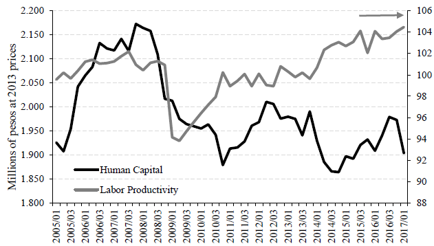
Source: Own elaboration based on Mulligan and Sala-i-Martin (1997) methodology, using data from INEGI.
Figure 3 Mexican Human Capital
Hence, in a broad definition, the measurement of human capital should cover formal and informal education, physical and mental skills, nutrition and social services that affect the quality of work.
Mulligan et al. (1997) propose to measure human capital as the average labor income in state i divided by the wage of workers with zero schooling in the same state:
This means that the quality of a person would be related to the wage rate received in the market. If the type of education that a person received was helpful, markets reward you with a high salary. Similarly, if a person is devoted to study a field that is not useful from the point of view of production, the productive human capital of that person would be low.
In order to capture all the components of human capital, in this study I use the methodology proposed by Mulligan et al. (1997). I use the average wage and the number of workers in order to obtain the average labor income, both variables are available at the National Survey of Occupation and Employment (ENOE, by its acronym in Spanish). I also assume that the salary of an unskilled person is equivalent to the minimum wage per day, which is available at the National Minimum Wage Commission. Notice that the estimated human capital that I obtained is consistent with the official estimation of labor productivity published by INEGI (see Figure 3). The relation between both variables seems to lose after the 2008-2009 financial crisis.
On the other hand, I used the System of National Accounts (SNA) in order to obtain data of GDP, consumption and capital. Additionally, I got data of GDP produced in the health sector, which is also available in the SNA, and data of schooling come from the ENOE. All data have a quarterly frequency, except the minimum wage, which have an annual frequency.3 Furthermore, all variables are seasonally adjusted with the official models of INEGI, meanwhile I adjusted the series from ENOE with the X13-ARIMA program.
Moreover, the model requires an approximation of the no-leisure time devoted to current production, 𝑢. To do this, I follow a similar methodology as Gong et al. (2004), that is; although it is recognized that the time devoted to human capital accumulation involves many years of schooling, work experience, etc.; the number of students across the country in a given school year is estimated as a fraction of total employment. The intuition is that, by using this ratio of the number of Mexicans who are studying, I capture the effect of those agents who spend time in education rather than going to work.
VEC Model for Human Capital
In response to the fact that the variable “human capital” constructed in this study does not distinguish between the contribution of education, experience or abilities, I propose a VEC model for human capital to identify solely the effect of education on economic growth.
Table 2 VEC Model of Human Capital
| Dependent Variable: DLOG(Human-Capital) | ||
| Method: Least Squares | ||
| Sample: 2006QII - 2016QIV | ||
| Variable | Coefficient | t-Statistic |
| LOG(Human-Capital(-1)) | -0.084*** | -3.30 |
| (0.024) | ||
| LOG(Schooling(-1)) | 0.342*** | 2.09 |
| (0.119) | ||
| LOG(Health(-1)) | -0.257** | -3.54 |
| (0.110) | ||
| DUMMY1304 | 0.028** | 7.03 |
| (0.011) | ||
| DUMMY1401 | -0.027** | -2.52 |
| (0.011) | ||
| DLOG(Human-Capital(-3)) | 0.189* | 1.91 |
| (0.099) | ||
| DLOG(Schooling) | 1.623* | 1.83 |
| (1.231) | ||
| DLOG(Schooling(-3)) | 0.888* | 1.79 |
| (0.689) | ||
| DLOG(Health(-2)) | 0.163*** | 2.77 |
| (0.059) | ||
| R-squared | 0.730 | |
| Adjusted R-squared | 0.622 | |
| S.E. of regression | 0.010 | |
| Durbin-Watson statistic | 1.867 | |
Standard errors in parentheses. ***p<0.01, **p<0.05, *p<0.1
Source: Author´s calculations.
In order to control for other variables that could influence human capital, I include in the model the GDP produced for the health sector, meanwhile I measure the education as years of schooling. On the other hand, notice that the GDP produced in health sector does not mean the accumulation of heath, on the contrary, it means the accumulation of sickness. Hence, I expect a positive sign for years of schooling but a negative sign for the variable “health”.
In my VEC model,4 the cointegration vector is represented by the (three) first variables in logarithms. Thus, I find that, in the long run, one percent increase in years of schooling produce a 0.342 percent increase in human capital (for quarterly growth rates). On the other hand, I find that a bad health abates the formation of human capital in a rate of 0.257 percent (see Table 2).
IV.Results
I find that solving the ULM with data from Mexico does not yield, in general, the
conventional parameters, which means that this model does not represents adequately
this developing economy. However, I imposed some restrictions to get results
consistent with the theory, i.e. I constrained:
Table 3 Uzawa-Lucas Model Estimation
| Parameters | Mexico/1 | USA/2 | Germany/2 |
|---|---|---|---|
| A | 1.01*** | 0.06*** | 0.05*** |
| (0.32) | (0.01) | (0.00) | |
| α | 0.38*** | 0.54*** | 0.48 |
| (0.08) | (0.13) | (0.36) | |
| ρ | 0.38** | 0.03*** | 0.01*** |
| (0.18) | (0.00) | (0.00) | |
| σ | 4.47*** | 1.55 | 0.40*** |
| (1.01) | (1.17) | (0.10) | |
| κ | 0.48*** | 0.07*** | 0.06*** |
| (0.18) | (0.00) | (0.01) | |
| ζ | 0.97*** | -0.01 | 0.01 |
| (0.31) | (0.07) | (0.39) | |
| Equations | DW Test | ||
| (8) | 1.8 | 1.9 | 1.9 |
| (9) | 1.8 | 1.8 | 2.0 |
| (10) | 1.7 | 1.3 | 0.9 |
| (11) | 2.3 | 0.2 | 0.3 |
/1 Results obtained using the Generalized Method of Moments (GMM) with Mexican data.
/2 Results from Gong et al. (2004) for their modified ULM.
Standard errors in parentheses. ***p<0.01, **p<0.05, *p<0.1
Source: Own calculations
Table 3 shows the results of the coefficients estimated from the ULM. Once I impose the afore mentioned restrictions, the coefficients’ magnitudes and signs are consistent with theoretical predictions. For example, the share of physical capital is roughly one third, just as the convention in literature. The elasticity of substitution, 1/σ = 0.22, is also consistent with the convention in macroeconomic models (Campbell and Mankiw [1989], and Lucas [2003]). The coefficient of the rate at which human capital accumulates, is positive and greater than the one estimated by Gong et al. (2004), κ = 0.48, which means that if individuals dedicated all their no-leisure time to the accumulation of human capital, this would increase in 0.48 percent. Additionally, the coefficient of human capital externality is also statistically significant, ζ = 0.97, unlike the one obtained by Gong et al. (2004).
The hypothesis that an increase in human capital increases production, is confirmed; indeed, I find that the increment in production is about 1.59 percent,5 once human capital increases in one percent. Thus, an increase of one percent in years of schooling causes an increase of the long run GDP growth rate of 2.19 percent.6 Notice that data of human capital has a quarterly basis, hence, the contribution of schooling in human capital (0.34) of Table 2 has an annualized rate of 1.38 percent.
Once I obtain the estimated coefficients, I proceed to analyze the model equilibrium at the steady state (Table 4). I find that, considering the positive externalities of human capital (ζ > 0), the GDP per capita equilibrium growth rate is 0.65 percent. Human capital grows at an annual rate of 3.03 percent, and per capita consumption grows at 1.67 percent. All those growth rates are consistent with a savings rate of 3.51 percent (for all these results I considered an annual population growth rate of 1.5 percent, which is the average growth rate in the period studied).
Table 4 Model equilibrium at the steady state
| Equilibrium steady state | ζ>0 | ζ=0 | |||
|---|---|---|---|---|---|
| Quarterly growth | Annualized growth | Quarterly growth | |||
| Growth rate of GDP per capita | ψ | 0.16 | 0.65 | 0.36 | 1.44 |
| Growth rate of human capital | ψ* | 0.75 | 3.03 | 0.36 | 1.44 |
| Growth rate of per capita consumption | γ | 0.41 | 1.67 | 0.36 | 1.44 |
| Savings rate | s | 0.87 | 3.51 | 0.95 | 3.84 |
Note: The growth rates at the steady state were computed using the ULM parameters estimated using the GMM.
Source: Own calculations.
Notice that since theory predicts sustained growth with or without externalities, we can now analyze the equilibrium at the steady state without externalities, i.e. ζ = 0; in that case, GDP per capita, human capital and consumption per capita grow at the same rate, i.e. an equilibrium annual growth rate of 1.44 percent, which is consistent with a savings rate of 3.84. These findings imply that the Mexican economy has a potential annual growth rate of 2.94 percent (1.44 of GDP growth + 1.5 of population growth). This means that, in 2016, the Mexican GDP growth was near its potential growth, but in 2017 the growth rate was 1.1 percentage points under its potential (Figure 4).

Conclusions
In this research I measure the effect of education on economic growth in a developing economy. For that purpose, I use Mexican time series to taste the Uzawa-Lucas Model (ULM) with the Generalized Method of Moments (GMM). Given that the ULM explains the influence of human capital on economic growth (but not the education on growth), I propose a VEC model of human capital in order to consider the indirect effect of education on the economic growth.
My results provide evidence that a rise of one percent in years of schooling increases human capital accumulation by 0.34 percent, on a quarterly basis, and at an annualized rate of 1.38 percent. Moreover, I find that an increase of one percent in human capital increases GDP by 1.59 percent. Thus, a rise of one percent in years of schooling causes an increase of the long run GDP growth rate of 2.19 percent. Additionally, based on the results of my VEC model, I conclude that a bad health abates the formation of human capital in a rate of 0.26 percent (on a quarterly basis).
Furthermore, omitting the effect of human capital externalities, I find that the Mexican economy has a potential annual growth rate of 2.94 percent. This result could be useful to policymakers (for example, as an additional estimation of the output gap, which is of interest for the Central Bank when taking monetary policy decisions) and as a reference to further research on the estimation of Mexican potential growth rate. Likewise, the parameters estimation that I have done in this research can also be used as a referent for future research, especially for the calibration of Macroeconomic models.
Finally, future research should consider two important issues that were not included in this paper. First, although I found that an increase in the educational attainment will increase the economic growth of Mexico, it is also true that my findings assume no changes in the quality of education. Improving the quality of education and rising the educational attainment would produce an even better effect on growth. Second, the segmentation of the Mexican labor market implies that an important proportion of workers considered in this research have a low productivity. Hence, since my results are based on an average of productive and unproductive workers, an increase of the years of schooling in each of both sectors is uncertain. My hypothesis is that increments of educational attainment in the productive (formal) sector would improve, even more, the economic growth of Mexican GDP.


