


 text new page (beta)
 English (pdf)
 Article in xml format
 Article references
 Send this article by e-mail
 Cited by SciELO
  Similars in
SciELO
Similars in
SciELO 
 Permalink
Introduction
Historically, Mexico has been an important player in oil production worldwide. The country reached its oil production peak in 2007 when it produced around 4.4 million barrels per day. With this production level, at the time, the country was the sixth largest oil producer in the world, after Saudi Arabia, Russia, the United States (U.S.), Iran, and China. However, this production level was not sustained, as in 2008 Mexico’s production started rapidly to decline. This led to the constitutional energy reform of 2013, introduced by President Pena Nieto (Campos 2016).
According to the International Atomic Energy Agency (2016) and the U.S. Energy Information Administration (2016), Mexico’s average oil production in 2016 was 2.19 million barrels per day. This placed the country in the position of the twelve largest oil producers worldwide. Oil prices are determined in dollars, and such an amount of oil produced assures that the government remains extremely dependent on oil revenues. The national income in U.S. dollars has had an effect on the Mexican peso exchange rate, and consequently also on other macro-economic variables in the country.
According to Lizardo and Mollick (2010) and Onour (2011), a severe drop in the oil price has been an important contributory factor in bringing on economic recession, increasing unemployment and inflation, and lowering the currency of oil-producing countries. Consequently, the Mexican central bank has to pay close attention to the oil price when it develops the country’s monetary policy. De Gregorio et al. (2007) shows important evidence about a decline in the pass-through effect from the oil price into the general price level. Among the factors that could help to explain such decline are a reduction in the exchange rate pass-through, a more favorable inflation environment, and some weaknesses related to the worldwide demand.
Given state dependence on the oil industry, variations in the oil price can have a big impact on the Mexican peso exchange rate, and eventually also on other macro-economic variables. Considering the importance of the MXN/USD exchange rate for the economy, our research aimed to investigate the impact of oil prices on the Mexican exchange rate. This paper differs from Lizardo and Mollick (2010) in that the research we report on refers exclusively to Mexico, uses a Vector Autoregressive Model (VAR), includes the spot and future oil prices as determinants of the exchange rate, and also pays attention to potential structural breaks across the analyzed period which spans 1991 to 2017.
Our first hypothesis is that besides the traditional variables included in the monetary model of exchange rates, the spot and future oil prices are additional factors that help to predict the spot MXN/USD exchange rate. The second hypothesis is that spot and future oil prices have different kinds of impact on the Mexican spot exchange rate. Arouri et al. (2012) include the spot oil price and future oil prices in their analysis, because the volatility in the spot and oil prices differs. This could be an important factor for better understanding the exchange rate variations.
The rest of the paper is structured as follows: section one describes the importance of the oil industry in the Mexican economy and its relation to the exchange rate. Section two provides an overview of the most relevant literature related to oil prices and exchange rates. Section three analyzes the data implemented in the model, and section four presents the methodology and the econometrics techniques implemented in the model. Section five describes the results, and the final section of this paper gives concluding remarks.
1. The Importance of Oil Revenue in the Mexican Economy
During the 1960s and 1970s Mexico’s annual inflation rate averaged around 3 percent, and the country maintained a good gross domestic product (GDP) growth rate. Such good results were partially due to high oil export revenue and to high government spending enabled by the import substitution model effective during that period. As a result, a substantial fiscal imbalance emerged and the country’s external debt increased considerably. Later, in the early 1980’s, oil prices plummeted, while world interest rates went up (Garcia 2001). This scenario created a great deal of stress in the Mexican economy which was highly dependent on oil revenue, and at the same time had incurred high debt in international markets. During that period, Mexico experienced a public debt crisis because the country was struggling to meet its external debt service requirements. Consequently, the government devaluated the peso three times in 1982, and the inflation rate reached values above 100 percent, as is shown in Figure 1.
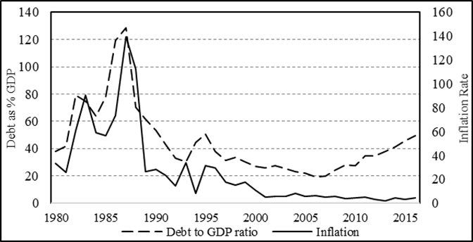
Source: Ministry of Energy (Mexican oil) and the U.S. Energy Information Administration (U.S. oil).
Figure 1: Government Debt Ratio and Inflation Rate, 1980-2016
The graph shows the inflation level and the government debt to GDP ratio in the Mexican economy for the period analyzed in this paper. As can be seen, the two variables have a similar path across the full period analyzed, indicating that government debt and inflation rate could be strongly related.
Garcia (2001) mentions that during the 1980s Mexico created a stabilization program to decrease the public debt, by focussing on fiscal reforms, trade openness, and increasing private investment. Lustig (1987) established that the reduction in public debt was accomplished by an increase in tax revenue and a decrease in public spending. During that period the Mexican economy entered a serious recession, so that between 1983 and 1988 the country’s GDP grew at an average rate of a mere 0.1 percent per year. For this reason, the 1980s are referred to as “the lost decade.”
Later, from 1988 to1994, the Mexican peso exchange rate was overvalued and controlled by the government, while the fiscal deficit increased considerably. In 1994, Mexico once again suffered a financial crisis, due mainly to an unexpected devaluation of the peso against the U.S. dollar. In 2001 the Banco de Mexico changed its monetary policy, setting the goal of keeping the inflation rate and growth expectations at low levels. This scheme reduced the pass-through effect from the exchange rate into the Consumer Price Index (CPI), as has been documented by Capistrán et al. (2012) and by Aleem and Lahiani (2013). In the following years the Mexican economy was stable, but in 2008 the country suffered another financial crisis, this time due to a mix of external and internal factors. Villarreal (2010) mentions that after the 2008 crisis, Mexico implemented a tax reform to replace oil revenue. Because Mexico had one of the lowest tax revenue to GDP ratios in Latin America, increasing tax revenues was likely to bring a decrease in dependence on oil.
Figure 2 shows the oil price trend across the period 1981 to 2017, and the percentage of oil revenue in the total government budget in the same period. As can be seen, oil revenue correlated highly with oil prices. Clearly higher oil prices provide the government with higher revenue, and vice versa. During the third quarter of 2016, oil constituted 11 percent of Mexico’s total export and around 15 percent of the government’s budget. Reyes and Benitez (2016), explained that over time the government had used these revenues to cover its current expenditures and maintain its fiscal balance. Campos (2016), mentioned that the oil sector had been instrumental in satisfying the government’s immediate needs, rather than increasing its long-term savings or the country’s wealth. This is referred to as a “hand to mouth policy.” Such governmental behavior would decrease the GDP and create economic problems when oil prices decrease.
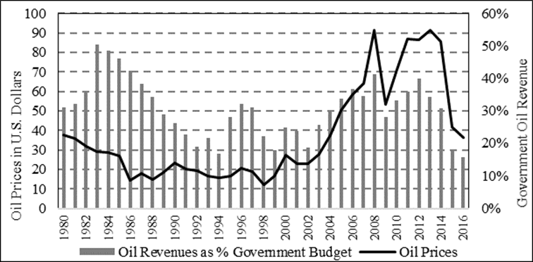
Source: Ministry of Energy (Mexican oil) and the U.S. Energy Information Administration (U.S. oil).
Figure 2: Oil Revenue as % Government Budget
Mexico’s 2015 government budget was based on a crude oil value of $79 per barrel, but in July 2015 the price was below $50 (Forbes, Mexico 2014). Then, in September 2015, Mexico’s federal government announced a cut in the PEMEX1 domestic investment, due to the drop in the oil price, which simultaneously reduced government oil revenue. Therefore, the federal government lowered government spending instead of increasing taxes or increasing the national debt. Since the MXN/USD foreign exchange rate is dependent on Mexico’s ability to export oil, the continued decrease in PEMEX’s output has left the company vulnerable (Wood 2017).
2. Previous Research
2.1 Oil Prices and their Effects on the U.S. Dollar
The relevant literature shows no consensus on the effect of a change in the oil price on the U.S. dollar price. Aloui, et al. (2013) analyze the conditional dependence structure between crude oil prices and the U.S. dollar exchange rate. They refer to a number of papers which found that an oil price increase is associated with a U.S. dollar depreciation. These papers include Wu, Chung and Chang (2012), Akram (2009), and Zhang, Fan, Tsai and Wei (2008). At the same time, there are papers which found that an oil price increase is associated with a U.S. dollar appreciation, such as Basher et al. (2012), Chen and Chen (2007), and Bénassy-Quéré, Mignon and Penot (2007).
Bloomberg and Harris (1995), in a study on the United States between 1970 and 1994, found evidence that commodity price movements, such as oil prices, are a reaction to swings in dollar exchange rates rather than to general inflation pressures. Later, Yoshino and Taghizadeh-Hesary (2014), in a study on the U.S. between 2007 and 2012, found that U.S. monetary policy strongly affects global oil prices. In other words, when the U.S. dollar depreciates, oil imports become cheaper in countries with weaker currencies, thus their demand for oil increases, as does the price of oil. In a different study on the U.S. economy, Abel, Bernanke and Croushore. (2008) shows that an increase in oil price is associated with a downward movement in oil production. Considering this, oil price changes are causally related to economic recessions.
Amano and Van Norden (1998) found that the real U.S. exchange rate and oil price variables were integrated. Their results show that according to Granger causality tests, oil prices cause the real exchange rate, but not vice versa. Additionally, Chen and Chen (2007) found that the real exchange rate could have been the source of its dynamics in the G-7 countries (which include the U.S.). They also developed a co-integration panel model to forecast the real exchange rates across countries. They found that real oil prices have significant forecasting power, and their predictability performance is more accurate over long-time periods.
Similarly, Basher et al. (2012) investigated the interaction between energy future prices and exchange rates. Their results show that future prices for crude oil, heating oil, and unleaded gasoline are integrated with a trade-weighted index of exchange rates. This means that there is a long-run equilibrium relationship between these four variables. Their results indicate that movement in the exchange rate precedes movement in oil future prices over time.
2.2 Oil Prices and their Effects on Currencies other than the U.S. Dollar
The Mexican economy strongly depends on the oil prices. Due to this, various studies have analyzed its correlation with the exchange rate. For example, Schwartz, Tijerina, and Torre (2002) discussed the volatility of the MXN/USD exchange rate, and found a positive relationship between the exchange rate and the oil price. They also found that if oil prices increase, Mexican terms of trade also increase, which in turn increases the real exchange rate and makes purchasing foreign goods more attractive.
Lizardo and Mollick (2010) added the oil price to a monetary model of exchange rates to explain the dynamics of the USD exchange rate. They found that when oil prices increase, the USD depreciates against the Mexican Peso and the currencies of other oil-exporting countries. Similarly, Volkov and Yuhn (2016) found that oil price shocks influence the level and volatility of the MXN/USD exchange rate. Their results also show that “the volatility of exchange rate changes is conditional on oil price changes.” Another finding is that the MXN/USD exchange rates take longer to reach their initial equilibrium than, for example, those of Norway and Canada.
Olomola and Adejumo (2006), in a study on oil-exporting Nigeria, show that oil price shocks are important determinants of the country’s exchange rate. They found that a high real oil price appreciates Nigeria’s home currency against other currencies. Akram (2004), although his results show a non-linear relationship between oil price and the Norwegian exchange rate, it holds only for the short run. This relationship is stronger when the oil price is below $14 U.S. dollars or when oil prices show a downward trend.
3. Data Analysis
The research data in this study comprise quarterly observations taken from 1991 to 2017. The estimated model includes macro-economic variables on the U.S. and Mexico, including their GDP, the MXN/USD exchange rate, money supply, and the spot and future oil prices.
The Mexican GDP is published by the National Institute of Statistics and Geography (INEGI) every quarter. The Mexican Central Bank (Banxico) provides the Mexican money supply rate (M1) and the exchange rate, respectively, on a monthly and daily basis. The Bureau of Economic Analysis (BEA) provides the U.S. GDP data every quarter, while the Federal Reserve Bank of St. Louis provides the U.S. money supply data every month. The Mexican money supply data (M1) is also available on a month basis, with the quarterly data comprising the average of each required quarter.
This paper introduces both the spot and the future oil prices into the econometric model because the volatility of each differs, and we hypothesize that this could affect the Mexican exchange rate in different ways. In our model, the spot oil price was obtained from the Bloomberg database on a monthly basis . The future oil price was obtained from the website investing.com, which provides the WTI2 future price of oil monthly, along with the quarterly data of each variable by calculating the average for each required quarter.
The exchange rate (fx) represents the percentage of change in the MXN per USD. The model includes the money supply (mt) of both the U.S. and Mexico, and the GDP (yt) for both economies. All these variables were converted into USD to ensure that all the analyzed variables are represented in the same currency. With respect to the last variable, the price of oil (log oil) used each year’s logarithm to obtain the price in real terms.
Table 1 displays the descriptive statistics of the analyzed variables. The nominal exchange rate value corresponds to the amount of pesos equivalent to one USD. The minimum value corresponds to 3.04 pesos per dollar in the first quarter of 1991, and the maximum value is 20.52 pesos per dollar in the last quarter of 2016.
Table 1 Descriptive Statistics
| Variable | Nominal Exchange Rate | Mexico GDP | U.S. GDP | Mexico M1 | U.S. M1 | Real Spot Price | Real Future Price |
|---|---|---|---|---|---|---|---|
| Mean | 10.32 | 819.04 | 12,269.59 | 93.45 | 1,621.42 | 43.11 | 51.65 |
| Median | 10.75 | 779.87 | 12,181.40 | 74.96 | 1,342.00 | 31.70 | 41.31 |
| Maximum | 20.52 | 1,340.10 | 19,500.60 | 216.60 | 3,556.70 | 114.50 | 140.91 |
| Minimum | 3.04 | 299.69 | 6,054.87 | 16.21 | 838.70 | 8.48 | 16.04 |
| Std. Dev. | 4.11 | 301.85 | 3,939.81 | 58.87 | 738.31 | 27.77 | 27.02 |
| Skewness | -0.05 | 0.00 | 0.07 | 0.53 | 1.26 | 0.89 | 0.83 |
| Kurtosis | 2.94 | 1.67 | 1.78 | 1.95 | 3.27 | 2.51 | 2.69 |
| Jarque-Bera | 0.06 | 7.92 | 6.73 | 9.94 | 28.70 | 15.14 | 12.81 |
| Probability | 0.97 | 0.02 | 0.03 | 0.01 | 0.00 | 0.00 | 0.00 |
Source: INEGI, Banxico, BEA, Federal Bank of St. Louis, Bloomberg and investing.com
The U.S. and Mexico’s GDP are given in billions of U.S. dollars and both values are in real terms (2008=100). The money supply (M1) of both countries is in hundreds of thousands (000,000) of U.S. dollars. Lastly, the values of the spot and future oil prices correspond to the dollar price per barrel. The minimum value corresponds to a spot oil price of $8.48 in October 1998, and the maximum value to $114.50 in April 2008. The maximum value of the future price is $140.91 in 2008.
4. Research Method
According to the traditional monetary exchange model, money supply is closely related to the inflation and exchange rates in a country. Rapach and Wohar (2002), in a study on 14 industrialized countries, use the simple long-run monetary model of the U.S. dollar exchange rate determination. Their results support the idea that in some of those industrialized countries, such a model is appropriate to understand the exchange rate dynamics.
As stated above, this paper uses a variation of the traditional monetary model of exchange rate determination, but also introduces the spot and future oil prices as potential exchange rate determinants for the Mexican peso. We hypothesize that the Mexican spot exchange rate not only reacts strongly to spot oil prices, but probably also to future oil prices. Cheung, Chinn and Pascual (2005) used the original monetary exchange rate model in their paper, but instead of oil prices, used other terms, such as trade, government debt, and the trade balance as determinants.
The model we implement assumes that the exchange rate is the relative price of two currencies, one of which is considered domestic money and the other foreign. Both types of monies have a demand which depends on each country’s price level, real income and interest rate. In addition, we assume that the Purchasing Power Parity (PPP) holds, meaning that prices are flexible. Lastly, our model assumes that the uncovered interest parity also holds between the countries. All these assumptions are discussed in detail in Lizardo and Mollick’s (2010) paper.
Finally, the implemented model works with the differences in the money supply from the home and the foreign country, repeating the process in terms of the GDP and adding oil prices as follows:
Where
Table 2 shows various unit root tests of the model’s variables. The Δ symbol represents the first difference in that variable. The tests performed, are the Augmented Dickey Fuller (ADF), Dickey Fuller Generalized Least Squares (DF-GLS) and Kwiatowksi-Phillips-Schimdt-Shin (KPSS). The ADF and DF-GLS tests assume that the null hypothesis has a unit root. The KPSS null hypothesis test assumes that the variable has a stationary trend. In the first two methodologies, the Schwartz Information Criterion is used to determine the lag selection, and the KPSS assumes that the series are stationary. If two out of three of the tests confirmed the presence of a unit root, then it is concluded that the series has a unit root.
Table 2 Unit Root Test Results
| Variable | ADF | L | DF-GLS | L | KPSS | L | Determination |
|---|---|---|---|---|---|---|---|
| (yt-yt*) | 1.679 | 1 | 2.010 2 | 2 | 1.174*** | 9 | I (1) |
| Log (yt-yt*) | -3.222*** | 0 | 0.817 | 3 | 1.163*** | 9 | I (1) |
| Δ Log (yt-yt*) | -4.870*** | 1 | -4.739*** | 1 | 0.453* | 7 | I (0) |
| (mt-mt*) | 6.634 | 0 | 2.874 | 2 | 0.9480*** | 9 | I (1) |
| Log (mt-mt*) | 1.100 2 | 2 | 2.038 2 | 2 | 1.031*** | 9 | I (1) |
| Δ Log (mt-mt*) | -4.162*** | 1 | -4.021*** | 1 | -4176* | 7 | I (0) |
| Nominal Exchange Rate | -0.738 | 0 | 1.111 | 0 | 1.174*** | 8 | I (1) |
| Log Nominal Exchange Rate | -1.854 | 0 | 0.820 | 0 | 0.968*** | 9 | I (1) |
| Δ Log Nominal Exch. Rate | -9.651*** | 0 | -9.511*** | 0 | 0.1935 | 3 | I (0) |
| Oil Real Spot Price | -1.940 | 0 | -1.191 | 2 | 0.838*** | 8 | I (1) |
| Log Real Oil Spot Price | -1.844 | 0 | -1.338 | 0 | 0.868*** | 9 | I (1) |
| Δ Log Real Oil Spot Price | -9.175*** | 1 | -9.572*** | 0 | 0.0783 | 3 | I (0) |
| Future Real Oil Price | -1.616 | 2 | -1.378 | 2 | 0.799*** | 8 | I (1) |
| Log Real Future Oil Price | -1.763 | 0 | -1.521 | 0 | 0.790*** | 9 | I (1) |
| Δ Log Real Future Oil Price | -8.969*** | 1 | -9.705*** | 0 | 0.087 | 2 | I (0) |
Note: The values reported are the statistical t values. Columns L refer to the selected lag length according to the Schwarz Criteria. The values in Column 7 use an automatic selection length of Newey-West bandwidth. Symbols *, **, *** indicate the rejection of the null hypothesis of the test corresponding to 10%, 5% and 1%, respectively.
When the log (mt-mt*), the log (yt-yt*), and the oil prices (spot and future) are first differentiated, all of them become stationary. Given the same integration order in the series, co-integration tests were carried out with the relevant variables of the study. Since some mt-mt* values are negative, the natural logarithm of these values is undefined. In such cases, the following algorithm is applied:
The same algorithm is applied for negative values in the log (yt-yt*). The Johansen (1988) trace and maximum eigenvalue tests are also implemented to check whether variables are co-integrated. If the variables in the econometric model are integrated, a Vector Error Correction Model (VECM) is required, otherwise a Vector Autoregressive Model (VAR) should be implemented.
Table 3 shows the results of both the basic and the composite models’ co-integration tests. The basic model is defined as follows:
Table 3 Johansen Co-integration Tests
| Model | Monetary Model | Composite (Spot Price) | Composite (Future Price) | |||
|---|---|---|---|---|---|---|
| Serie | fx, (mt-mt*), (yt-yt*) | fx, (mt-mt*), (yt-yt*) Log (Spot Price) | fx, (mt-mt*), (yt-yt*) Log (Future Price) | |||
| Test | Statistic | Prob. | Statistic | Prob. | Statistic | Prob. |
| Trace Statistic | ||||||
| None | 30.36* | 0.04 | 52.65* | 0.01 | 51.80* | 0.02 |
| At most 1 | 15.36 | 0.05 | 30.78* | 0.03 | 29.04 | 0.06 |
| At most 2 | 4.18* | 0.04 | 15.25 | 0.05 | 14.60 | 0.06 |
| At most 3 | 5.04* | 0.02 | 5.63* | 0.01 | ||
| Max Eigen Statistic | ||||||
| None | 14.99 | 0.29 | 21.86 | 0.22 | 22.76 | 0.18 |
| At most 1 | 11.17 | 0.14 | 15.53 | 0.25 | 14.44 | 0.33 |
| At most 2 | 4.18 | 0.04 | 10.21 | 0.19 | 8.96 | 0.28 |
| At most 3 | 5.03 | 0.02 | 5.63 | 0.01 | ||
Note: * denotes rejection of the hypothesis at the 5% level.
While the composite model is the one already defined to test our hypothesis (Equation 1), the only difference between the two models is in the log (oil price) in the composite model. This paper hypothesizes that oil is a significant factor beyond the classic monetary model in explaining variations in the Mexican exchange rate against the U.S. dollar.
Results of Johansen's co-integration tests show that there is no long-term relationship in the models. However, this conclusion may not be entirely clear given the results listed in Table 3. To reinforce the results, an Engle-Granger co-integration test that was additionally run, is included in the Appendix. Although, Table 3 could leave some doubt about the presence of a long-term relationship in the models, the table included in the Appendix which shows the Engle-Granger cointegration test results, confirms the non-existence of co-integration of the analyzed variables. The Granger causality test indicates the variables that should be considered as endogenous, as well as the variables that should be considered as exogenous in the empirical model. The results of the causality tests are shown in Table 4.
Table 4 Granger Causality/Block Exogeneity Wald Tests
| Sample: | 1991Q1 2017Q3 | ||
| Included observations: | 105 | ||
| Dependent variable: Δ Log Nominal Exchange Rate | |||
| Excluded | Chi-sq | df | Prob. |
| Δ Log Real Spot Oil Price | 5.10 | 1 | 0.02 |
| Δ Log Real Future Oil Price | 9.24 | 1 | 0.00 |
| All | 10.57 | 2 | 0.01 |
| Dependent variable: Δ Log Real Spot Oil Price | |||
| Excluded | Chi-sq | df | Prob. |
| Δ Log Nominal Exchange Rate | 0.00 | 1 | 0.96 |
| Δ Log Real Future Oil Price | 2.03 | 1 | 0.15 |
| All | 2.03 | 2 | 0.36 |
| Dependent variable: Δ Log Real Future Oil Price | |||
| Excluded | Chi-sq | df | Prob. |
| Δ Log Nominal Exchange Rate | 0.04 | 1 | 0.85 |
| Δ Log Real Spot Oil Price | 0.10 | 1 | 0.75 |
| All | 0.13 | 2 | 0.94 |
Source: Authors’ own with data from Banxico, Federal Bank of St. Louis and investing.com
The results show that only the nominal exchange rate is Granger-caused by spot oil price and future oil prices. In both cases, the null hypothesis of non-causality is rejected at a level of 99% confidence.
Therefore, for the period in question, the evidence tends to support the use of only one dependent variable in the VAR model, which is:
Where
5. Results
Table 5 displays the regression results of the VAR model for the period analyzed in this paper. The possible existence of auto-correlation in the model was tested using the Lagrange Multiplicator (LM) test. Results give evidence that there were no auto-correlation problems in the regression. LM tests about auto-correlation are also included in the Appendix.
Table 5 VAR model
| Variables | Δ Log Nominal Exchange Rate |
|---|---|
| Δ Log Nominal Exchange Rate (-1) | 0.106 |
| (0.110) | |
| Constant | -0.367 |
| (0.001) *** | |
| Δ Log (yt-yt*) | -36.182 |
| (0.000) *** | |
| Δ Log (mt-mt*) | -6.544 |
| (0.010) ** | |
| Δ Log Spot Oil Price | -0.780 |
| (0.094) * | |
| Δ Log Future Oil Price | -0.153 |
| (0.424) | |
| D1995 | -0.534 |
| (0.057) * | |
| D2008 | 1.070 |
| (0.002) *** |
Note: P values in parenthesis
Source: Authors’ own with data from INEGI, Banxico, BEA, Federal Bank of St. Louis, Bloomberg and investing.com
Results in Table 5 indicate that the difference between the growth rates of the Mexican and the U.S. money supplies is statistically significant. Estimates also show that when the Mexican money supply grows faster than the U.S. money supply. The model thus predicts a depreciation of the MXN against the USD. The interpretation is the same, and statistically significant, when the U.S. economy grows faster than the Mexican GDP does. Results further show an inverse and significant relationship between spot oil prices and the Mexican spot exchange rate, indicating that an increase/decrease in the oil price creates an appreciation/depreciation in the Mexican peso. Finally, estimated outcomes also indicate that future oil prices are not statically significant in the model.
To put the results of the study into the bigger picture, the impulse-response functions derived from the VAR model appear in Figure 3. Figures 3a and 3b show the impulse response functions for the effects on the nominal exchange rate based on changes in the spot and future oil prices. Results indicate that a positive shock in the spot oil price creates an appreciation on the exchange rate in the following 3 months, after which it decreases until it vanishes.

Note: Response to Cholesky One S.D. Innovations ± 2 Standard Errors.
Figure 3: Impulse-Response Functions
Regarding future oil prices, results indicate an immediate effect in the first month, after which the price decreases, and then, seven months after the initial shock, disappears. The future oil price shock, compared to the spot oil price shock, is transmitted into the nominal exchange rate more dynamically. The corresponding appreciation of the nominal exchange rate leads to a decrease in the foreign capital flow, until subsequently, the effect vanishes.
The next kind of shock to be examined, is an unanticipated increase in the exchange rate, shown in Figures 3c and 3d. As expected, the responses of spot and future oil prices to an increase in the nominal exchange rate, are similar. Both respond negatively in the first month, and such effect gradually disappears in the following months. Lastly, Figure 3e shows the response in future oil price to a positive shock in spot oil price. We observe a big response during the first two months, when the spot price increases significantly, and after the third month the effect vanishes. Figure 3f shows that the effect of the future oil price on the spot price is close to zero from the first month onwards.
Summary and Concluding Remarks
That Mexico has been largely dependent on oil revenue, is indicated by oil sales at the end of 2016 representing approximately 15 percent of the government's budget income. Oil prices4 have consistently been an important causal factor in Mexican peso exchange rate variations. Given the importance of the oil price in determining the exchange rate, this study has focused on analyzing the impact of the spot and future oil prices on the estimation of the MXN/USD exchange rate from 1991 to 2017.
Unit root tests have been run, as well as the appropriate co-integration and causality tests. In addition, structural break tests were performed, indicating structural breaks in 1994, 2008 and 2011. The 2011 structural break was dropped from the regressions because results were not statistically significant. Results indicate that a VAR model was appropriate for the estimations.
The first hypothesis in this paper assumes that besides the traditional variables included in the monetary model, the spot and future oil prices play an important role in Mexican peso exchange rate variations, and therefore also help to explain such variations. Results obtained in the paper confirm the hypothesis. Basically, we found that increases/decreases in the spot oil prices create an appreciation/depreciation in the spot value of the Mexican peso against the U.S. dollar. The second hypothesis assumes that future oil prices also play an important role in determining the Mexican spot exchange rate. Our estimates do not support this hypothesis. The results indicate that future oil prices are not statistically significant in explaining variations in the Mexican peso exchange rate. In addition, we also found that to assure Mexican peso stability, the Mexican money supply and GDP should grow at a similar rate to the equivalent variables in the U.S. economy.
Importantly, one has to mention that government revenue in Mexico has to reduce its dependency on the oil industry, in order to reduce the Mexican peso’s dependency on oil price fluctuation. Our results indicate that oil reforms implemented in Mexico in 2013 could, indeed, in the long run reduce the volatility of the Mexican Peso. Additional reforms which can help the Mexican economy to become more competitive, are encouraged.

