


 text new page (beta)
 English (pdf)
 Article in xml format
 Article references
 Send this article by e-mail
 Cited by SciELO
  Similars in
SciELO
Similars in
SciELO 
 Permalink
Introduction
During the last three decades (1987-2017), global financial markets have experienced several crises: 1987 stock market crash, 1994 Mexican crisis, 1997 Asian crisis, 1998 Russian crisis, 2001 dot com crisis, 2007-2008 subprime crisis and 2009-2012 global financial crisis. These episodes have been characterized by negative asset returns and high volatility levels in foreign exchange and stock markets, particularly in the case of emerging markets. Indeed, risk associated with international portfolios has increased due to: i) stock returns expressed in domestic currency are affected through changes in the exchange rate movements and ii) negative shocks affecting one market could be transmitted to other markets, generating contagion effects.
The strong relationship between stock prices and exchange rate movements not only impacts portfolio decisions, but it also alters economic policies, investment appraisal and funding costs. Theoretically, currency depreciation improves competitiveness on local firms enhancing exports and future cash flow. However, generally, emerging markets import more than they export and a currency depreciation has a negative impact in their terms of trade, increasing the cost of capital and raw materials, reducing competitiveness of local firms. Thus, stock prices will rise (diminish) in response to increases (decreases) in expected cash flows.
An extensive body of empirical literature has explored the dynamic linkages between stock prices and exchange rate movements. For instance, Beer and Hebein (2008) use an Exponential General Autoregressive Conditional Heteroskedasticity (EGARCH) framework to explore the relationship between stock prices and exchange rates for two groups of countries: emerging and developed economies. Their evidence yields some positive significant price spill over effects from the foreign exchange market to the stock market in Canada, Japan, the U.S and India. Their findings also show that there is no persistence of volatility in the stock markets and the exchange rate markets, in developed countries, but the volatility is pronounced and enduring in emerging countries. Tsai (2012) estimates the relationship between stock price index and exchange rate in six Asian countries; the methodology employed is the quantile regression model. Results show that a negative relation between stock and foreign exchange markets is more obvious when exchange rates are extremely high or low. Liang, Lin and Hsu (2013) examine the relationships between the equity market and currency market in the ASEAN-5 using the panel Granger causality and panel dols methodologies. Their results suggest that exchange rates impact stock prices negatively via capital mobility
On the other hand, Walid, Chaker, Masoodk and Fry (2011) analyse the dynamic linkage between stock price volatility and exchange rate changes for four emerging countries over the period 1994-2009, employing the Markov-Switching EGARCH model. They provide evidence signalling that the relationship between stock and foreign exchange markets are regime dependent and stock-price volatility responds asymmetrically to events in the foreign exchange market. Additionally, their findings suggest that foreign exchange rate changes have a significant impact on the probability of transition across regimes. Chkili and Nguyen (2014) use a regime switching VAR model approach to investigate the dynamic linkages between the exchange rates and stock market returns for the BRICS countries. Their result shows that stock markets have more influence on exchange rates during both calm and turbulent periods.
Among the studies about Latin American countries, Romero-Meza, Bonilla, Benedetti and Serletis (2015) analyse financial contagion employing bicorrelation test to graphically represent non-linear events detected in Latin American stock markets. Their results show that contagion caused by financial crises induces nonlinear dependencies. Maya, Albeiro, Gomez-Gonzalez & Melo Velandia (2015) use vine copula methodology to evaluate the level of contagion among six Latin American countries. Their findings suggest that there is contagion effect in Latin America in periods of large appreciations.
Kanas (2005) explores the issue of volatility regime linkages between the Mexican currency market and six emerging equity markets by using Markov Switching Vector Autoregressive model (MS-VAR). He contributes evidence of regime dependence between the Mexican currency market and each one of these equity markets.
Following inquires in the literature, this paper employs the MS-VAR model to analyse the dynamic linkages between the stock market returns and the exchange rate changes on the equity markets of Latin American Integrated Market (MILA): Colombia, Chile, Mexico and Peru, which represents the largest Latin-American market, with a combined market capitalization of about $1 trillion of usd and nearly 1,000 issuers, surpassing Brazil´s stock market. In order to test the hypothesis that, stock and foreign exchange markets have a dynamic relation. This study is not only important to investors and portfolio and currency hedge managers; it is also of utmost importance to policy makers who are concerned about the crises transmission and its effects on investment and economic growth. The MS-VAR model is proposed to evidence the connections between the foreign exchange (FX) and stock markets. This model was selected based on its advantages. One of the main features of the Markov-switching process is their ability to model the asymmetry, non-linearity and persistence of extreme observations (Anas, Billio, Ferrara and Duca, 2004); these characteristics are proper of financial and economic series. In turn, the MS-VAR model presents a more general formulation than the linear VAR. At the same time, it provides the basis to test independence without splitting the sample, giving a more accurate correlation coefficient, which is based in not arbitrarily partitioned subsamples (Kanas, 2005). The period of study covers from 2003:01 to 2016:09, including the subprime crisis and the global financial crisis. It allows justifying the application of Markov regime switching model because, according to several studies, stock markets and exchange rate movements are closely related during regime-shift episodes.
The paper is organized as follows. The next section presents the methodology used to estimate the dynamic linkages between stock and FX markets. Section 2 describes the data. Section 3 presents and analyses the results, finally conclusions are presented.
1. Methodology
A time-series variable y t can be modelled by a Markov switching autoregressive of order p (MS-AR), with regime shifts in mean and variance. It is represented as follows (Hamilton, 1989)
where φ i is the autoregressive coefficients µ and σ are the mean and standard deviation depending on the regime s t at the time t, y t represents the stock market returns of the MILA countries. This MS-AR model detects potential regime shifts in the stock market returns and enables to estimate the impact of crises on the stock market volatility (Chkili and Nguyen, 2014).
The aim of this study is to analyse the dynamic relationship between the equity market and the FX market of the MILA countries. For this purpose, is advanced the Markov Switching Vector Autoregressive model developed by Krolzig (1997). This model is a generalization of the MS-AR presented above and can be written as follows:
where r t and e t represent the stock market and exchange rate returns for each country, respectively, υ t is the innovation process with a variance v(s t ) depending on regime s t which is assumed to follow an irreducible ergodic two-state Markov process, defined by the transition probabilities p ij between states as follows:
where,
The MS-VAR model provides an accurate estimation of the potential regime shifts in the stock and exchange rate returns, above all, during the turbulent period analysed in this study. The inclusion of structural breaks in the financial time-series analysis is crucial to avoid mistaken conclusions related to the dynamic behaviour of stock and currency markets and their relationships.
2. Data
2.1 MILA Performance
As previously mentioned, MILA is the largest Latin-American capital market; its performance from 2011 to 20161 is described in Table 1. It is important to point out that over this period Latin American markets experienced the Global Financial Crisis effects. Accordingly, it can be observed that MILA capitalization has decreased, in absolute (23.6%) and in relative terms (46% as GDP percentage).
Table 1 MILA General Data
| 2011 | 2012 | 2013 | 2014 | 2015 | 2016 | ||
| Chile | GDP (Bill us) | 219.28 | 231.14 | 240.66 | 245.16 | 250.58 | 254.40 |
| GDP Growth | - | 5.4% | 4.1% | 1.9% | 2.2% | 1.5% | |
| Issuing companies | 200 | 272 | 227 | 230 | 224 | 217 | |
| Capitalization (Bill us) | 258.67 | 313.46 | 266.01 | 233.04 | 190.60 | 209.86 | |
| Capitalization (%GDP) | 107.8% | 118.1% | 95.7% | 90.1% | 79.1% | 82.5% | |
| Capitalization Growth | - | 21.2% | -15.1% | -12.4% | -18.2% | 10.1% | |
| Colombia | GDP (Bill US) | 293.08 | 304.94 | 319.80 | 333.85 | 344.04 | 350.78 |
| GDP Growth | - | 4.0% | 4.9% | 4.4% | 3.1% | 2.0% | |
| Issuing companies | 83 | 84 | 81 | 74 | 73 | 71 | |
| Capitalization (Bill us) | 201.58 | 272.81 | 120.65 | 153.08 | 88.00 | 104.00 | |
| Capitalization (%GDP) | 60.0% | 70.9% | 53.3% | 38.8% | 29.4% | 29.6% | |
| Capitalization Growth | - | 35.3% | -55.8% | 26.9% | -42.5% | 18.2% | |
| México | GDP (Bill us) | 1065.36 | 1105.62 | 1123.41 | 1148.88 | 1179.12 | 1203.32 |
| GDP Growth | - | 3.8% | 1.6% | 2.3% | 2.6% | 2.1% | |
| Issuing companies | 140 | 134 | 143 | 159 | 238 | 137 | |
| Capitalization (Bill US) | 504.00 | 525.00 | 535.70 | 480.96 | 401.00 | 352.00 | |
| Capitalization (%GDP) | 34.9% | 44.2% | 41.7% | 37.0% | 35.2% | 33.3% | |
| Capitalization Growth | - | 4% | 2% | -10% | -17% | -12% | |
| Peru | GDP (Bill US) | 152.59 | 161.66 | 171.02 | 175.22 | 181.01 | 188.11 |
| GDP Growth | - | 5.9% | 5.8% | 2.5% | 3.3% | 3.9% | |
| Issuing companies | 273 | 258 | 282 | 275 | 173 | 280 | |
| Capitalization (Bill US) | 113.58 | 153.40 | 120.65 | 120.76 | 91.00 | 124.00 | |
| Capitalization (%GDP) | 47.7 | 53.3 | 40.3 | 39.2 | 29.9 | 48.2 | |
| Capitalization Growth | - | 35.1% | -21.3% | 0.1% | -24.6% | 36.3% | |
| MILA | Market capitalization | 936.27 | 1062.76 | 975.67 | 873.54 | 712.03 | 715.46 |
| Annual variation | - | 28.9% | -31.4% | -0.1% | 40.0% | 11.3% | |
| Capitalization (%GDP) | 89.3% | 70.1% | 46.6% | 39.4% | 48.2% | ||
| Issuing companies | 696 | 748 | 733 | 738 | 746 | 705* |
GDP and Market Capitalization (%GDP) Data were obtained from World Bank Data (2017). Issuing companies and Market Capitalization Data were obtained from MILA market annual reports. * Own estimation.
It is also important to mention that, above all, during 2013 the market capitalization fell by 31.4%. Another important fact is the annual variation of issuing companies, which can be attributed to regulation and taxation changes in each local market.
Analysing local patterns, the Peruvian market is the only one that has experienced a relative and absolute growth since MILA consolidation. Colombian, Mexican and Chilean markets have decreased their capitalization in 48%, 30% and 19%, respectively. This analysis reveals a negative trend in MILA since its creation; it could be partially explained by the international financial uncertainty.
2.2 Descriptive Statistics
To test the dynamic relationship between the stock and exchange rate returns, daily closing prices of stock indexes in local currency (Colombia- COLCAP, Chile-IPSA, Peru-IGBVL and Mexico-IPC), and bilateral exchange rates (national currency unit per US dollars) are employed. The data period is from January 1, 2003 to September 29, 20162 (3,585 observations). The stock index data are extracted from the web site yahoo finance and the exchange rate data are obtained from International Monetary Fund Data Base. Daily returns are estimated by taking the difference in the logarithm of two consecutive prices.
Descriptive statistics of MILA countries equity and exchange rate (XR) markets are presented in Table 2. Standard deviation, mean and unit root tests are included. The mean of stock indexes is higher than the mean of the exchange rate for all the markets under analysis, except the Colombian one which could be explained by the 2006 Colombian peso depreciation process. Stock markets present higher volatility than XR, Chilean market is the least volatile (1.1%), followed by Mexican (1.3%), Colombian (1.4%) and Peruvian market (1.7%).
Table 2 Descriptive Statistics in levels and returns
| Country | Series | Mean | Std Dev | ADF | PP | ||||
| Levels | Returns | Levels | Returns | Levels | Returns | Levels | Returns | ||
| Colombia | Stock returns | 6.8913 | 0.0007 | 0.6452 | 0.01400 | -3.3905* | -47.8584* | -1.9134 | -50.989* |
| XR changes | 7.7017 | 0.0000 | 0.1819 | 0.00822 | -1.3220 | -44.1048* | -1.2804 | -43.968* | |
| Mexico | Stock returns | 10.1656 | 0.0007 | 0.5810 | 0.01334 | -2.6805*** | -38.6156* | -1.2249 | -49.905* |
| XR changes | 2.52835 | 0.0002 | 0.1505 | 0.00741 | 0.1207 | -50.9921* | 0.6239 | -50.989* | |
| Chile | Stock returns | 7.99712 | 0.0005 | 0.4128 | 0.01144 | -3.2849** | -46.9462* | -1.8684 | -46.820* |
| XR changes | 6.32375 | -0.0000 | 0.1305 | 0.00718 | -1.8552 | -45.8974* | -1.9671 | -45.868* | |
| Peru | Stock returns | 9.23508 | 0.0008 | 0.7695 | 0.01709 | -1.8128 | -45.0241* | -1.8094 | -46.282* |
| XR changes | 1.11074 | -0.0000 | 0.0940 | 0.00319 | -1.280879 | -46.3070* | -1.3291 | -46.304* | |
Reported values are statistical significance levels of * 1%,** 5% and 10% ***.
The condition of stationarity is checked applying the Augmented Dickey Fuller and Phillips Perron tests. Results suggest that the null hypothesis about the presence of a unit root is rejected; values of stock indexes and exchange rates are greater than the critical MacKinnon value at a 1 % level. Therefore, it is confirmed that the series are stationary in returns.
3. Results
3.1 Testing for Volatility Regime Switch Behaviour
To examine the dynamic relationship between stock and exchange rate markets, it is essential to confirm that MILA stock markets present regime-switching behaviour. The log likelihood test (LR) is employed to test the null hypothesis the data set is homoscedastic, against the alternative hypothesis of, regime switching model (MS-AR) reproduces better the stock markets behaviour (Garcia and Perron, 1996). This test is estimate as follows
where lnL is the log likelihood of the contrasting models. The best-fitted model is selected through Davies (1987) critical values. This test has been used in several studies (Kanas, 2005; Wang and Theobald, 2008; Chkili and Nguyen, 2014) to prove that other emerging markets exhibit a time-varying behaviour, which responds to local circumstances and to the effects of crises transmission. To reinforce the tests results, it is also introduced the Akaike Information Criteria (AIC). Table 3 shows the results of both tests.
Table 3 LR and AIC tests statistics results
| LnL(AR) | LnL(MS-AR) | LR | AIC (AR) | AIC(MS-AR) | |
| Colombia | -4782.699 | -4282.555 | 1000.288* | 3.505274 | 3.142531 |
| Chile | -4224.702 | -3810.351 | 828.702* | 3.096485 | 2.796594 |
| Mexico | -4657.454 | -4256.485 | 801.938* | 3.41352 | 3.123432 |
| Peru | -5306.132 | -4658.031 | 1296.202* | 3.888741 | 3.417605 |
Reported values are statistical significance levels of * 1%
Source: Own estimation with the estimation results
Table 3 indicates that the log-likelihood value of the MS-AR is significantly higher than the linear AR model in all the markets. The rejection of the null of no-volatility regime switch is equivalent to the rejection of the ar in favour of the alternative MS-AR model. The Akaike Information Criterion (AIC) endorses this results; it is also in favour of the MS-AR model in all cases.
3.2 MS-AR Results
Once that regime-switching behaviour is proved in stock markets returns, the MS-AR models are estimated; their results are described in Table 4. Standard deviations (σ1 2 and σ2 2) are statistically significant at 1% and their values suggest the presence of two regimes. The first regime is a low volatility level while the second regime presents a high volatility level. For all the markets, the standard deviation of the high volatility regime is at least the double of the low volatility regime. Chile and Colombia exhibit the highest volatility level in the low volatility regime, and Peru presents the highest volatility in the high volatility regime.
Table 4 MS-AR Model Results
| Colombia | Chile | Mexico | Peru | |||||
| Const(1) | 0.0948* | (0.0223) | 0.0876* | (0.0197) | 0.1193* | (0.0214) | 0.1069* | (0.0268) |
| Const(2) | -0.0102 | (0.0196) | -0.1028 | (0.1076) | -0.1277* | (0.1044) | -0.0021 | (0.0069) |
| AR1 | 0.1140* | (0.0199) | 0.130698* | (0.0199) | 0.0554* | (0.0190) | 0.1672* | (0.0198) |
| σ1 2 | 0.2290* | (0.0317) | 0.301686* | (0.0228) | 0.0855* | (0.0196) | 0.0661* | (0.0224) |
| σ2 2 | 0.8924* | (0.0417) | 0.726864* | (0.0452) | 0.8816* | (0.0391) | 1.1093* | (0.0356) |
| P11 | 0.951739 | 0.970247 | 0.987033 | 0.97613 | ||||
| P22 | 0.852619 | 0.879717 | 0.942425 | 0.922981 | ||||
| d1 | 20.72065 | 33.6095 | 77.11606 | 41.89376 | ||||
| d2 | 6.785148 | 8.313741 | 17.36877 | 12.98377 | ||||
Reported values are statistic significance levels of * 1%,** 5% and 10% ***. Standard deviations are reported in parentheses.
Source: Own estimation with the estimation results
Table 4 also presents the probability of being in each regime. As expected, the probability of being in a high volatility regime (P 22) is lower than the probability of being in the low volatility regime (P 11), in all cases. This evidences the fact that low volatility regime is more persistent than the high volatility regime. Mexico is the country with the highest level of persistence in both low (0.942) and high volatility regime (0.987) followed by Peru (P 11=0.922, P 22= 0.976), Chile (P 11=0.879, P 22=0.970) and Colombia (P11=0.852, P 22=0.951).
Results of the average duration for each regime (d 1 and d 2) confirm the presence of two regimes. The average duration of the high volatility regime (d 2) is 17.36 days for Mexico, 12.98 days for the Peruvian market, 8.31 days for Chile and 6.78 days for the Colombian market. In contrast, the average duration of the low volatility regime (d 1) is in Mexico 77.11 days, Peru 41.89 days, Chile 33.60 days and Colombia 20.72 days.
3.3 Graphic Analysis: Index, Stock Market Returns and Smooth Probabilities
Figure 1 present the index in levels, stock market returns and the smooth probabilities of being in regime 2 (high volatility regime). All the indexes present a positive trend with an important fall in 2009, apparently, due to the global financial crisis effect. The stock market returns series exhibit volatility clusters, asymmetry and persistence in the volatility, above all, in periods associated with financial disequilibria.
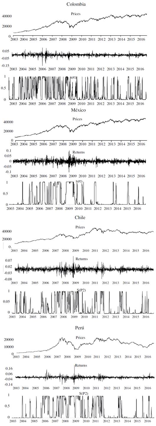
Source: Own estimation with the estimation results.
Figure 1 Index, Stock Market Returns and Smooth Probabilities
The smooth probability of being in the high volatility regime (S (P2)) indicates the presence of several common high volatility episodes which stands in out some periods: 2007-2008 (subprime crisis), 2009 (global financial crisis) and 2011-2012 (sovereign debt crisis). The smooth probability graphs show that the Colombian and Chilean markets are constantly getting in and out of the regime 2. It could indicate that these markets are very sensitive to local and international financial shocks. The case of the Peruvian market is similar to the Colombian and Chilean markets, but the Peruvian market has been in and out only during 2006 to 2012. It evidences that the subprime crisis, the global financial crisis and the sovereign debt crisis had important effects on the Peru stock market.
The Mexican market from 2005 to 2008 was getting in and out of the high volatility regime, but in 2009 it gets in this regime and stayed there the whole year. Afterwards, the Mexican market presented some peaks in different periods. In general, all the stock markets under study present non-coincident peaks among them, that could be related to local patterns associated with decisions of policy makers, macroeconomic variables and business and economic cycles.
3.4 MS-VAR Results
The exchange rate is a key variable to determine the real rate of return, above all in international portfolio investments; because of that, its behaviour keeps a close relation to the stock market behaviour. This relation, particularly, increases during crises episodes. In this sense, this paper aims to analyse the dynamic linkages between the stock and the exchange rate markets employing a MS-VAR model. To begin with, it is necessary to determine the lag length. Based on Likelihood Ratio (LR) tests of alternative lengths, a lag length of 1 was chosen to estimate the model. In second place, the LR and AIC tests are applied to demonstrate that regime-switching behaviour exists in the linkages of stock and exchange rate markets, results are presented in Table 5.
Table 5 LR and AIC tests statistics results
| LnL(var) | LnL(MS-VAR) | LR | AIC (var) | AIC(MS-VAR) | |
| Colombia | -4782.699 | -4281.742 | 1001.91* | 3.506007 | 3.144133 |
| Chile | -4224.097 | -3808.923 | 830.34* | 3.096774 | 2.797746 |
| Mexico | -4646.821 | -4249.187 | 795.26* | 3.406462 | 3.120284 |
| Peru | -5306.067 | -4657.629 | 1296.87* | 3.889426 | 3.419509 |
Reported values are statistic significance levels of * 1%
Source: Own estimation with the estimation results
Results shown in Table 5 prove that LR tests reject the null hypothesis of no regime switching in the relationship between stock market and exchange rate returns in all cases; it means that the alternative MS-VAR is the more-suitable model. The Akaike Information Criterion (AIC) is also in favour of the MS-VAR model in all cases. Hence, MS-VAR is estimated, the results are in Table 6.
Table 6 Stock and exchange markets: MS-VAR model results
| Colombia | Chile | Mexico | Peru | |||||
| α1 | 0.0814* | (0.0201) | 0.0740* | (0.0173) | 0.1129* | (0.0204) | 0.0876* | (0.0217) |
| α21 | 0.1333* | (0.0257) | 0.1475* | (0.0238) | 0.0518* | (0.0219) | 0.1780* | (0.0257) |
| α22 | 0.0639 | (0.0698) | 0.06734 | (0.0483) | -0.0580 | (0.0467) | 0.1405* | (0.0558) |
| α31 | 0.0091 | (0.0074) | -0.018851 | (0.0298) | -0.0480 | (0.0325) | -0.0209 | (0.0053) |
| α32 | -0.0079* | (0.0016) | -0.056419 | (0.0925) | -0.3968* | (0.1151) | 0.1047 | (0.0786) |
| β1 | 0.0247 | (0.0488) | 0.0238 | (0.0320) | 0.1207* | (0.0371) | 0.0118 | (0.0166) |
| β21 | -0.1978* | (0.0228) | 0.1023* | (0.0398) | -0.0318 | (0.0336) | 0.1290** | (0.0653) |
| β22 | -0.0520* | (0.0086) | 0.1165* | (0.0228) | -0.0297 | (0.0282) | 0.0925** | (0.0276) |
| β31 | 0.1465* | (0.0296) | -0.1551* | (0.0315) | -0.0860* | (0.0233) | 0.0043 | (0.0106) |
| β32 | 0.1423* | (0.0278) | -0.0985* | (0.0127) | -0.0110 | (0.0099) | 5.87E-05 | (6.59E-05) |
| P11 | 0.9520 | 0.9730 | 0.9870 | 0.9764 | ||||
| P22 | 0.8534 | 0.9125 | 0.9427 | 0.9236 | ||||
| Average duration | ||||||||
| Regime 1 | 20.8357 | 33.06002 | 77.19413 | 42.44639 | ||||
| Regime 2 | 6.824344 | 8.327768 | 17.47821 | 13.10135 | ||||
| Std deviation stock markets | ||||||||
| Regime 1 | 0.228593 | 0.305173 | 0.086271 | 0.064401 | ||||
| Regime 2 | 0.891098 | 0.72051 | 0.867832 | 1.109557 | ||||
| Std deviation exchange rate | ||||||||
| Regime 1 | 0.135164 | 0.112459 | 0.076377 | 0.659529 | ||||
| Regime 2 | 0.936409 | 0.692338 | 0.799198 | 2.271266 | ||||
| Correlation coeficient | ||||||||
| Regime 1 | -0.632328543 | -0.472480986 | 0.700641257 | -0.740359081 | ||||
| Regime 2 | -0.565482139 | -0.556992282 | 0.068209945 | -0.863234846 | ||||
Reported values are statistic significance levels of * 1%,** 5% and 10% ***. Standard deviations are reported in parentheses.
Source: Own estimation with the estimation results.
The standard deviation of the stock markets and exchange rate markets is lower in regime one (low volatility regime) than in regime two (high volatility regime), for all the markets. It indicates the presence of two different volatility regimes. The probability that a day of low volatility will be followed by a day of low volatility (transition probability P 11) is 0.987 for Mexico, 0.976 for Peru, 0.973 for Chile and 0.952 for Colombia. On the other hand, the probability that a day of high volatility will be followed by a day of high volatility (transition probability P 22) is 0.942 for Mexico 0.923 for Peru, 0.912 for Chile and 0.853 for Colombia. The average duration of low volatility regime is of 77.19 days for Mexico, 42.44 days for Peru, 33.06 days for Chile and 20.83 days for Colombia.
Table 6 also reports the correlation coefficient between stock and exchange rate markets in low and high volatility regimes. In the case of Chilean and Peruvian market correlation is negative and absolute values are higher during the high volatility regime than during the low volatility regime. This finding is similar to the results of Kanas (2005), Lin (2012) and Chkili and Nguyen (2014). This evidence has been interpreted as a contagion effect between asset prices. It is important to point out that, Mexican market is the only one that presents positive correlation, but during high dependence regime it is very low (0.06) in comparison to the low dependence regime. It means that, when there is contagion effect, the stock and foreign exchange markets are not correlated.
The estimated coefficients capturing the impact of exchange rate movements on stock market returns (α31 and α32) are not significant in all cases, except for the Peruvian market. It suggests that the US dollar variations do not have an important effect on stock markets’ behaviour.3 This result also coincides with the findings of other studies (Kanas, 2000; Yang and Doong, 2004; Aloui, 2007 and Chkili and Nguyen, 2014). On the other hand, the coefficients (β31 and β32) capture the effects of stock market returns on exchange rate movements. They are statistically significant in the case of Colombia, Chile and Mexico, but insignificant for Peru. This relation is negative in high and low level of volatility for the Mexican and the Chilean market, suggesting that in these markets an increase in stock market returns leads to appreciation of the respective exchange rate (Chkili and Nguyen, 2014). This result is consistent with previous studies (Chkili and Nguyen, 2014; Hatemi-J and Roca, 2005; Pan et al, 2007 and Granger et al, 2000).
Conclusion
This paper examines the dynamic linkages between the stock and exchange rate markets in MILA countries: Colombia, Chile, Mexico and Peru, over the period 01:2003-09:2016. The empirical evidence of the MS-AR model suggests that all the stock markets display a switching regime behaviour, presenting two different levels of volatility: a high volatility regime and a low volatility regime. The high volatility regime exhibits less persistence than the low volatility regime. In this sense, the hypothesis is accepted.
The smooth probabilities of being in the high volatility regime show the presence of several common high volatility episodes in dates close to the financial disequilibria occurrence. In the case of Colombia, Chile and Peru markets present high sensitivity to local and international shocks.
On the other hand, MS-VAR is employed to analyse the dynamic relationship between the stock market returns and the exchange rate movements. This financial relation also evolves according to two different volatility regimes: high and low volatility levels, for all the markets under study. Findings suggest that stock markets have influence on exchange rate, but the exchange rates do not have a significant impact on stock markets. Results for the Peruvian and Chilean markets constitutes evidence about contagion between the stock and the exchange rate markets.
These findings shed some light about the relationship between two of the most important financial markets in a dynamic and complex international financial environment. Portfolio investors and currency hedge managers could take this information to develop international investment strategies that include MILA stock markets, forecasting results in two different scenarios: high and low volatility. On the other hand, policy makers could take this information to anticipate exchange rate movements as a consequence of changes in stock market behaviour. Further research may apply this method to analyse dynamic linkages between other financial markets (commodities, debt, equity and foreign exchange markets) in other developed and emerging countries, to contrast results and contribute evidence about financial relationships.

