


 text in
  English (pdf)
 Article in xml format
 Article references
 Send this article by e-mail
 Cited by SciELO
  Similars in
SciELO
Similars in
SciELO 
 Permalink
Introduction
Evapotranspiration includes the loss of water from crops by transpiration and from the soil by evaporation, making it a key variable in the development of irrigation schedules and the optimization of water resources (Santiago-Rodríguez et al., 2018). Evapotranspiration occurring on a vegetated surface is a function of the meteorological conditions of the area and the anatomical and physiological characteristics of vegetation (Allen et al., 1994).
The evapotranspiration rate of a reference area that occurs without water restrictions is called reference evapotranspiration (ETo). This area corresponds to a hypothetical grass or alfalfa crop (with specific characteristics). It is assumed that the only factors affecting it are meteorological parameters to be calculated from atmospheric weather measurements (Allen et al., 1998). ETo can be measured with direct methods such as lysimeters, eddy-covariance towers, evapotranspirometers and evaporimeter tanks (Mauder et al., 2018). Alternatively, estimated with indirect or empirical methods usually obey equations or models obtained by regression. In the first case, specialized equipment and qualified personnel are required for management, which is costly and makes implementation difficult in agricultural areas.
Among the empirical methods for estimating ETo, the FAO modified Penman-Monteith method (PMMF) stands out for its accuracy (Allen et al., 1998). However, this method is limited to compact geographic areas. It requires a large amount of meteorological data (Toro-Trujillo et al., 2015), such as relative humidity, wind speed and solar radiation, often unavailable at conventional stations in Mexico (Lavado et al., 2015). An alternative is to use less sophisticated empirical methods with more affordable meteorological variables and extrapolate point values to large extensions using the spatial interpolation methods (Aragón-Hernández et al., 2019; Greenough & Nelson, 2019). Indirect ETo estimates allow filling the missing information gap around this meteorological variable of great agriculture importance.
Chihuahua, located in the north of Mexico, is a state with an arid and semi-arid climate with an average precipitation of 252 to 482 mm-yr-1 (Instituto Nacional de Estadística y Geografía [INEGI], 2017), making water a scarce resource. Despite these conditions, about 597 000 ha are cultivated under irrigation and 443 000 ha under rainfed. The main irrigated crops are cotton (with 166 000 ha in the spring-summer cycle) and grain wheat (with 8 000 ha in the autumn-winter period) (Servicio de Información y Estadística Agroalimentaria y Pesquera [SIAP], 2018).
The extensive agricultural areas of Chihuahua are cultivated under irrigation in irrigation districts and units, where water volume designation is the responsibility of the Comisión Nacional del Agua (CONAGUA). Each year, irrigation water demand is calculated from ETo estimates made with empirical methods; subsequently, these estimates are extrapolated to the rest of the agricultural area without considering spatial variation, which results in errors and overestimates. Some ETo estimates made with the PMMF method suggest that Chihuahua values range from 100 to 270 mm-month-1 (Ruíz-Álvarez et al., 2014) or from 3.5 to 8.5 mm-day-1 (Lozoya et al., 2014), with the highest values in June.
Campos-Aranda (2005) estimated that ETo values in Chihuahua range from 60 mm-months-1 in January to 200 mm-months-1 in June, with an R2 of 0.96 when comparing Hargreaves-Samani with PMMF. These values indicate a strong demand for water resources in this region, aggravated in agricultural areas by high water consumption and low irrigation water application efficiency.
Despite the efforts described above to understand and meet the water needs of crops in the state of Chihuahua, the low availability of climatic information is a limitation for quantifying and analyzing the spatiotemporal variation of ETo. Accurate ETo estimates incorporating spatio-temporal variation contribute to improving water resource allocation, especially in agricultural areas where the resource is scarce. It is essential to achieve a more efficient use. In this sense, the objective of this study was to analyze the spatio-temporal variation of ETo estimated from empirical methods and spatial interpolation, using meteorological observations available for the state of Chihuahua.
Materials and methods
Study area
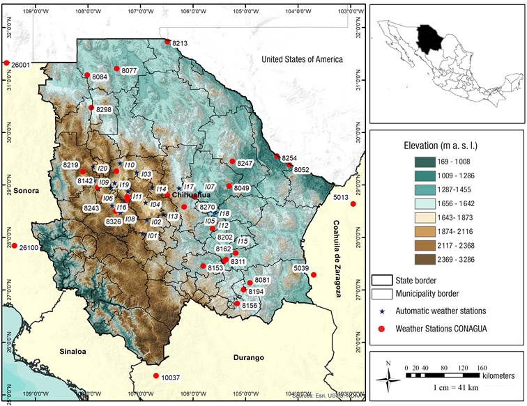
The state of Chihuahua is located in the north-central region of Mexico (31° 47' 04" and 25° 33' 32" north latitude, and 103° 18' 24" and 109° 04' 30" west longitude). Chihuahua represents 12.6 % of the national territory, is bordered to the northeast by the United States of America, to the east by Coahuila de Zaragoza and Durango, to the south by Durango and Sinaloa, and to the west by Sonora and Sinaloa (Figure 1). The territory has four types of climates: very dry (40 %), dry and semi-dry (33 %), temperate-sub-humid (24 %) and warm-sub-humid (3 %). The average annual temperature is 17 °C, and the average annual precipitation is 500 mm (INEGI, 2017).
Meteorological data and processing
Daily temperature and precipitation records were obtained from 33 meteorological stations managed by the Servicio Meteorológico Nacional (SMN) (CONAGUA-SMN, 2019) for the period 1960-2013 (Figure 1, Table 1). This data series includes outlier data cleaning, which is performed by SMN staff. Data were subjected to the double mass curve test, where each station was compared to surrounding stations for consistency, as recommended by Gao et al. (2017), Ruíz-Álvarez et al. (2020) and Searcy and Hardison (1960), and all measurements were consistent. A homogeneity test was also performed using the PROCLIMDB package developed for the R program (Štěpánek et al., 2009), which works similarly to CLIMATOL (Guijarro, 2016). This analysis showed that climatic information from all the stations used is homogeneous.
Table 1 Weather stations used in the study.
| ID | Name | X | Y | Elevation (m a. s. l.) |
|---|---|---|---|---|
| 8004 | Bachiniva | 279793 | 3184779 | 2 017 |
| 8044 | Delicias (DGE) | 454499 | 3118802 | 1 173 |
| 8049 | Luis L. León | 469634 | 3205655 | 1 080 |
| 8052 | El Mulato | 580642 | 3251948 | 774 |
| 8059 | El Tintero | 261240 | 3239694 | 2 450 |
| 8077 | Guzmán | 266606 | 3456205 | 1 200 |
| 8081 | Jiménez (DGE) | 508255 | 3001202 | 1 370 |
| 8084 | Ascensión (DGE) | 784950 | 3444124 | 1 323 |
| 8085 | La Boquilla | 459332 | 3046747 | 2 119 |
| 8099 | Majalca | 355108 | 3187042 | 1 155 |
| 8102 | Meoqui (DGE) | 452598 | 3126841 | 1 932 |
| 8142 | Temosachi (OBS) | 225463 | 3205714 | 1 290 |
| 8153 | Valle de Zaragoza (DGE) | 420266 | 3037025 | 1 350 |
| 8156 | Villa Coronado | 484089 | 2957493 | 1 516 |
| 8162 | Camargo (DGE) | 481928 | 3063984 | 1 250 |
| 8185 | Presa Chihuahua (DGE) | 385906 | 3162376 | 1 548 |
| 8194 | Villa López | 496418 | 2986779 | 1 424 |
| 8202 | Presa Francisco I. Madero | 438397 | 3115883 | 1 242 |
| 8213 | Juárez (DGE) | 359194 | 3512179 | 1 135 |
| 8215 | Las Chepas | 280632 | 3178510 | 2 076 |
| 8219 | Peñitas | 782536 | 3239399 | 2 135 |
| 8243 | Tejolocachi (DGE) | 236606 | 3184348 | 1 920 |
| 8247 | Coyame (DGE) | 475756 | 3257869 | 1 220 |
| 8254 | Ojinaga (DGE) | 558128 | 3269074 | 800 |
| 8270 | La Mesa | 405939 | 3183250 | 1 250 |
| 8298 | Dublan | 218328 | 3375014 | 1 440 |
| 8311 | Colina | 463341 | 3050423 | 1 214 |
| 8326 | Presa Abraham González | 258236 | 3155235 | 2 000 |
| 5039 | Sierra Mojada | 628631 | 3018733 | 1 256 |
| 10037 | La Huerta, Topia | 328890 | 2806268 | 670 |
| 26001 | Agua Prieta | 638065 | 3466622 | 1 210 |
| 26100 | Tesopaco, Rosario | 657804 | 3080602 | 421 |
| 5013 | Ejido San Miguel | 700550 | 3169454 | 1 060 |
| I01 | Buena Vista, Carichi* | 308057 | 3105965 | 1 719 |
| I02 | Campo 26, Cuauhtémoc* | 315657 | 3135074 | 1 749 |
| I03 | Campo 305, Namiquipa* | 298403 | 3236198 | 1 947 |
| I04 | Campo 8, Cuauhtémoc* | 314138 | 3172065 | 1 782 |
| I05 | El Paraíso, Aldama* | 434628 | 3154251 | 1 443 |
| I06 | Faciatec, Namiquipa* | 250714 | 3204783 | 1 849 |
| I07 | Inifap Aldama, Aldama* | 415367 | 3192047 | 1 290 |
| I08 | La Junta, Guerrero* | 266883 | 3151677 | 1 976 |
| I09 | La Tiznadita, Temósachi* | 219898 | 3220682 | 1 602 |
| I10 | Las Cruces, Namiquipa* | 268152 | 3256147 | 2 239 |
| I11 | Las Varas, Bachíniva* | 281690 | 3196628 | 2 000 |
| I12 | Lázaro Cárdenas, Meoqui* | 441162 | 3139876 | 1 534 |
| I13 | Loma Verde, Cuauhtémoc* | 347006 | 3146728 | 1 546 |
| I14 | Maurilio Ortiz, Cuauhtémoc* | 326212 | 3204248 | 1 610 |
| I15 | Puerto de Toro, Saucillo* | 476856 | 3093180 | 1 401 |
| I16 | Rancho Colorado, Guerrero* | 251374 | 3167218 | 1 956 |
| I17 | Sacramento, Casas Grandes* | 376813 | 3201513 | 1 356 |
| I18 | Salón de Actos, Rosales* | 442634 | 3151532 | 1 477 |
| I19 | Soto Mainez, Namiquipa* | 257343 | 3214490 | 1 969 |
| I20 | Sta. Clara, Namiquipa* | 218046 | 3250400 | 1 995 |
*Automated weather stations (AWS)
Relative humidity and wind speed records were collected from 20 automatic weather stations (EMAs), managed by the Instituto Nacional de Investigaciones Forestales, Agrícolas y Pecuarias (INIFAP), for the latest available period (1 to 3 years) (INIFAP, 2019). These records were used to validate the relative humidity values required to operate the PMMF method. Finally, solar radiation was calculated using the equation described by Allen et al. (1998).
The missing values of databases were estimated with the interpolation method known as inverse distance weighted (IDW), according to Equation 1 (Shepard, 1968):
Where Zp is the estimated value for the point, n is the number of points used in the interpolation, Z i is the known meteorological record, d i is the distance between stations (m), and p is the power depending on the degree of terrain undulation: 1 for flat and 2 for steep.
Empirical methods for calculating reference evapotranspiration
The empirical methods used to calculate ETo were selected based on the availability of meteorological information in the study area. Table 2 shows the empirical methods used to calculate ETo. The reference method was PMMF, while the methods compared or evaluated were Hargreaves (Hg), Turc (Tc), Blaney Criddle (BC), Thornthwaite (Th), Malmstrom (Mm), Makkink (Mk) and Hargreaves modified by Droogers (Dg).
Table 2 Empirical methods for estimation of reference evapotranspiration (ETo).
| Method | Variables | Equation | Reference |
|---|---|---|---|
| Hg | Tmx, Tmn Tm, R a |
|
Hargreaves & Samani (1985) |
| Tc | Tm, R G |
|
Turc (1961) |
| BC | Tm |
|
Doorenbos y Pruitt (1977) |
| Th | Tm |
|
Thornthwaite (1948) |
| Mm | Tm |
|
Malmström (1969) |
| Mk | Tmx, Tmn, R S |
|
Makkink (1957) |
| Dg | Tprom, TD, P, R a |
|
Droogers & Allen (2002) |
| PMMF | Tm, Hr, Vv, R n |
|
Allen et al. (1998) |
Tmn = minimum temperature (°C); Tmx = maximum temperature (°C); Tm = mean temperature (°C); Tprom = daily average temperature (°C); TD = daily temperature range (°C); P = precipitation (mm·month-1); a and b = empirical constants; C = relative humidity dependent constant; R G = global radiation (MJ·m-2·day-1); R S = solar radiation (MJ·m-2·day-1); R a = extraterrestrial radiation (MJ·m-2·day-1); R n = net radiation (MJ·m-2·day-1); G = heat flux (MJ·m-2·day-1); p = annual mean percentage of daylight hours; d = number of days per month; I = annual heat index; γ = psychrometric constant (kPa·°C-1); Δ = slope of the saturated vapor stress curve (kPa·°C-1); u 2 = wind speed at 2 m height (m·s-1); e s - e a = vapor stress deficit (kPa).
Statistical analysis
Comparison of means of each empirical method regarding the reference method (PMMF) was performed with an analysis of variance (P ≤ 0.05) and by the Tukey-Kramer least significant difference (LSD). The hypotheses tested were: HO) the mean values of each empirical method is equal to that of the reference method. HA) at least one mean value of the empirical methods is different from that of the reference method. A linear regression analysis was performed between the values of each empirical method against those of the reference method. In this case, the hypotheses tested were HO) the slope of the regression line is equal to 0 and HA) the slope of the regression line is different from 0. The precision was evaluated with the coefficient of determination (R2), root mean square error (RMSE), mean error (ME) and the Nash-Sutcliffe efficiency (NSE) calculated according to Equations 2 to 5 (Alexandris et al., 2006; Cervantes-Osornio et al., 2012; Djaman et al., 2018; Nash & Sutcliffe, 1970; Tabari, 2010).
where a
i
is the value estimated by the empirical method, t
i
is the value obtained with the reference method, ā is the average of the estimates with the empirical method,
Spatial and temporal analysis
The geographic information was organized in a Geographic Information System (GIS) with QGIS software ver. 3.8 "Zanzibar". The IDW method was used to obtain regular interpolated surfaces of monthly, seasonal, and average annual values of meteorological variables and ETo with a 1 km x 1 km pixel size. A spatio-temporal analysis of ETo values was performed with the maps obtained, including precipitation and temperature spatial and temporal distribution. Due to the volume of information generated in this study, only the annual and seasonal maps: spring (March-May), summer (June-August), autumn (September-November) and winter (December-February), are shown.
Results and discussion
This section includes a brief analysis of the spatial and temporal characteristics of temperature and precipitation in the state of Chihuahua to highlight the relationship between these variables and ETo. ETo values obtained, their statistical analysis, and spatiotemporal distribution are shown.
Temporal analysis of precipitation and temperature
Figure 2 shows the maximum and minimum average annual temperature and the annual cumulative precipitation for 1960-2013. The maximum temperature in this period ranged from 28.5 °C (2011) to 25 °C, while the minimum temperature was between 10.7 and 7.7 °C (1973). On the other hand, the average annual cumulative precipitation was 270 mm; the highest value was in 2004 (493 mm) and the lowest in 1960 (55 mm).
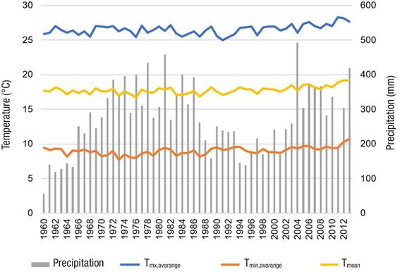
Figure 2 Mean annual temperature and annual cumulative precipitation in Chihuahua, Mexico (1960-2013).
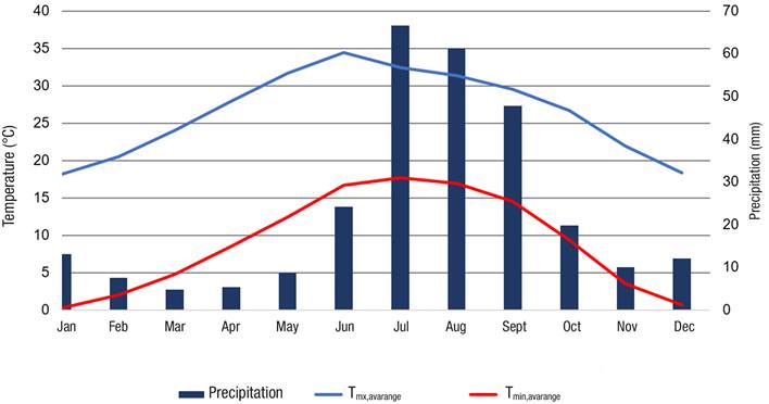
Chihuahua shows a monomodal cycle concerning temperature and precipitation (Figure 3). The average maximum temperature ranged from 18 °C in January to 34.4 °C in June, while the minimum temperature varied from 0.3 °C in January to 17 °C in July. The highest monthly average precipitation was in July (66.6 mm), and the lowest value (4.8 mm) was recorded in March. The figure shows that the high-temperature season coincides with the rainy season (June-September). The dry season coincides with low temperatures (October-March); therefore, the planning of sowing and harvesting is necessary.
Spatial distribution of temperature and precipitation
Chihuahua is the largest state in Mexico, which generates significant differences in the distribution of temperature and precipitation. Figure 4 shows the spatial distribution of temperatures (maximum and minimum) and average seasonal rainfall in the state. The maximum temperature (36.5 °C) occurs in summer in Ojinaga (800 m a. s. l.), while the minimum (14.2 °C) happens in winter in Maderas (2 110 m a. s. l.). Therefore, agriculture is mainly carried out in the spring-summer cycle (May-October).
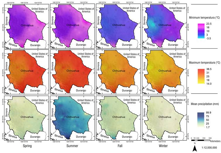
Figure 4 Spatial distribution of seasonal temperature (maximum and minimum) and precipitation in Chihuahua (1960-2013).
In Chihuahua, temperature decreases at a rate of 6 °C per 1 000 m ascent, according to the linear regression model in Figure 5a (R2 = 0.74). Temperature varies from 34 °C at 169 m a. s. l. to 15 °C at 3 286 m a. s. l.
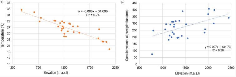
Figure 5 Linear regression between elevation (m a. s. l.) versus a) mean annual temperature (°C) and b) cumulative annual precipitation (mm) in weather stations of the Comisión Nacional del Agua (CONAGUA) in Chihuahua, Mexico.
Regarding precipitation, the maximum value was for the municipality of Bachiniva (99 mm, 2 017 m a. s. l.), while the minimum was in spring in Ojinaga (1.7 mm, 770 m a. s. l.). It is estimated that in 75 % of the state's surface, the annual cumulative precipitation is less than 300 mm, with a gradient that increases from east to west: from 73 mm in the region adjacent to the United States to a maximum of 552 mm in the Sierra Madre Occidental.
The precipitation-height relationship is complex. Figure 5b shows the model obtained by linear regression of this relationship. The R2 value was 0.28 (P ≤ 0.05), with a precipitation gradient increasing at a rate of 9.7 mm per 1 000 m of ascent. This relationship, although low, indicates that precipitation could be influenced by other variables, such as terrain relief and slope, especially in mountainous regions (Geng et al., 2017).
Reference evapotranspiration values
The statistical parameters (mean, standard deviation, quartiles) and outliers of ETo allows comparing the methods used and studying their frequency distribution. The diagrams in Figure 6 show the variation of the average daily ETo calculated with the eight empirical methods, which indicate a mean ranging from 2.5 to 5.3 mm·day-1 and a standard deviation between 1 and 2.2 mm·day-1. The PMMF method reached an average value of 5.3 mm·day-1, with a standard deviation of 2.2 mm·day-1. The Dg and Hg methods are the closest to PMMF, with a mean of 5.2 and 4.5 mm·day-1, respectively; this represents underestimating ETo values of 2 and 15 % concerning PMMF. This coincides with that reported by Allen et al. (1998). They indicate that the methods that come closest to PMMF consider temperature and radiation as the primary sources of energy that promote evapotranspiration, like Hg and Dg.
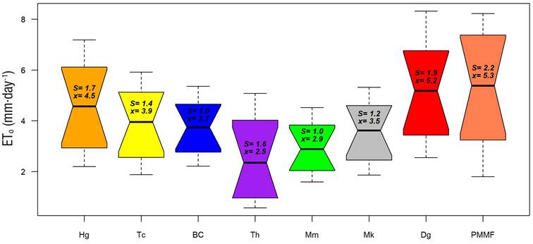
Figure 6 Box plot for reference evapotranspiration (ETo) values estimated from eight empirical methods.
The methods with the lowest dispersion were Mm (1.5 to 4.5 mm·day-1) and BC (2.2 to 5.3 mm·day-1), which coincides with that reported by Le et al. (2012), who indicate that in regions with high variation of climate, height and land use conditions, empirical methods do not always provide satisfactory results. PMMF and Dg methods had the highest values of standard deviation (S) (2.2 and 1.9 mm·day-1, respectively), while Mm and BC had the lowest values of S (1.0 mm·day-1, in both cases).
Statistical analysis
The comparative statistical analysis between the empirical methods identified the closest methods to the reference method (PMMF). Table 3 and Figure 7 show the analysis of variance for the comparison of means and linear regression between ETo values estimated by empirical methods and the PMMF reference method. The comparison of means shows that, except for the Dg method, the empirical methods show statistically significant differences (P > 0.05) concerning PMMF. In the case of linear regression, all methods showed a statistically significant linear relationship with the PMMF method.
Table 3 Results of comparison of means and linear regression of reference evapotranspiration (ETo) values between empirical methods (Hg, Tc, BC, Th, Mm, Mk and Dg) and the reference method (Penman-Monteith modified by FAO [PMMF]).
| Method | Comparison of means | Linear regression | ||||||||||||
|---|---|---|---|---|---|---|---|---|---|---|---|---|---|---|
| Mean (µ) | S | C. I. for the mean | Difference of means | C.I. for the difference of means | Slope | C.I. for the slope | R2 | RMSE | ME | NSE | ||||
| Lower | Upper | Lower | Upper | Lower | Upper | |||||||||
| Dg | 5.24 a | 1.96 | 5.09 | 5.39 | 0.04 | -0.22 | 0.31 | 0.93* | 0.89 | 0.97 | 0.70 | 1.23 | -0.97 | 0.68 |
| Hg | 4.59 b* | 1.71 | 4.46 | 4.72 | 0.70 | 0.43 | 0.96 | 0.64* | 0.62 | 0.67 | 0.83 | 1.16 | -0.69 | 0.71 |
| Tc | 3.91 c* | 1.40 | 3.80 | 4.01 | 1.38 | 1.11 | 1.64 | 0.67* | 0.65 | 0.70 | 0.83 | 1.73 | -1.38 | 0.37 |
| BC | 3.73 cd* | 1.05 | 3.65 | 3.81 | 1.56 | 1.29 | 1.82 | 1.30* | 1.28 | 1.32 | 0.78 | 2.02 | -1.55 | 0.14 |
| Mk | 3.58 d* | 1.19 | 3.49 | 3.67 | 1.70 | 1.44 | 1.96 | 0.85* | 0.83 | 0.87 | 0.81 | 2.11 | -1.74 | 0.06 |
| Mm | 2.94 e* | 1.01 | 2.86 | 3.02 | 2.34 | 2.08 | 2.61 | 0.61* | 0.59 | 0.63 | 0.68 | 2.72 | -2.34 | -0.55 |
| Th | 2.54 f* | 1.62 | 2.42 | 2.67 | 2.74 | 2.48 | 3.00 | -1.18* | -1.21 | -1.15 | 0.76 | 2.94 | -2.74 | -0.81 |
Dg = Hargreaves modified by Droogers; Hg = Hargreaves; Tc = Turc; BC = Blaney Criddle; Mk = Makkink; Mm = Malmstrom; Th = Thornthwaite; S = standard deviation; R2 = coefficient of determination; RMSE = root mean square error; ME = mean error; NSE = Nash-Sutcliffe efficiency; C.I. = confidence interval. Letter indicates statistical difference group; * indicates statistically significant differences (LSD, P < 0.05) in the comparison of means and that the linear regression is statistically significant.
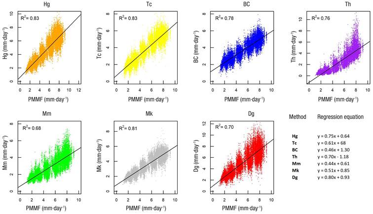
Figure 7 Linear regression between the seven empirical methods and Penman-Monteith method modified by the FAO (PMMF). Hg = Hargreaves; Tc = Turc; BC = Blaney Criddle; Th = Thornthwaite; Mm = Malmstrom; Mk = Makkink; Dg = Hargreaves modified by Droogers.
All methods had R2 values above the minimum value (0.70) reported by Moriasi et al. (2007), indicating a good fit concerning the reference method. RMSE values ranged from 1.2 to 2.9 mm·day-1, while ME ranged from -0.7 to -2.7 mm·day-1and NSE went from -0.55 to 0.71; this suggests that all methods underestimated ETo calculated with PMMF. The results obtained agree with those reported by Lozoya et al. (2014). The method closest to PMMF was Hg with R2 = 0.83, RMSE = 1.1632 mm·day-1, ME = -0.695 mm·day-1, NSE = 0.71. It can be an alternative to calculate ETo in regions where only temperature records are available, as in Chihuahua, since the value of extraterrestrial radiation can be obtained from tables or with the equation recommended by Allen et al. (1998). However, if solar radiation measurements, wind speed, temperature and humidity are available, it would be feasible to use PMMF (Lozoya et al., 2014).
The comparative analysis shows that the methods that consider temperature and radiation (Hg, Tc, BC, Th and Mk) performed better regarding PMMF than those using temperature and other variables such as relative humidity and precipitation (Mn and Dg).
Analysis of monthly reference evapotranspiration
A comparative analysis of the average daily values of ETo on a monthly scale, estimated with the different empirical methods, shows that all the methods studied have similar results throughout the year, although with significant differences depending on the season (Figure 8). According to the results, the maximum ETo values occur between June and July (4.5 to 8.3 mm·day-1), and the minimum between January and December (0.5 to 2.5 mm·day-1). Six methods underestimate PMMF most of the year with values ranging from 0.1 to 4.1 mm·day-1 (Hg, Tc, BC, Th, Mm and Mk). The months with the most considerable differences concerning PMMF (between 2 and 4 mm·day-1) are in the rainy spring and summer seasons (February and October), while the minor differences (< 2 mm·day-1) correspond to late autumn and early winter (November, December and January) (Figure 8), which is in agreement with that reported by Ayyoub et al. (2017). The Dg method is the only one that overestimates PMMF almost throughout the year, except in July, August, and September.
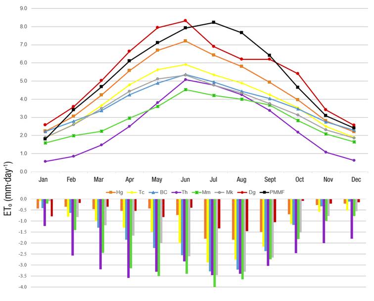
Figure 8 Temporal monthly distribution of reference evapotranspiration (ETo) estimated with empirical methods and differences concerning the reference method (Penman-Monteith, modified by the FAO (PMMF).
The most significant differences concerning PMMF occur in June with values ranging from 1.3 to 4.1 mm·day-1, while the minor differences (0.2 to 1.8 mm·day-1) occur in December and January. The closest to PMMF is Hg and Dg, with differences ranging from 0.1 to 1.8 mm·day-1. These extremes occur in December and August, respectively, indicating that the most significant differences are concentrated in the months when the temperature begins to decrease, coinciding with the rainy seasons, similar to that obtained by Lozoya et al. (2014). These results indicate that estimating ETo closest to the reference method (PMMF) on a monthly scale is Hg. It was used throughout the state to obtain homogeneous surfaces of monthly, seasonal and annual values.
Spatial distribution of seasonal reference evapotranspiration
The spatial interpolation of point values of ETo in areas where there is no climate information allows the elaboration of maps to analyze spatial variation. Figure 9 shows seasonal average maps generated from the spatial interpolation of daily ETo calculated with the Hg method. The highest ETo values were reported in the spring (5.6 to 7.1 mm·day-1) and summer (4.9 to 6.5 mm·day-1), increasing from higher to lower elevations in a west-east direction. The highest ETo value (7 mm·day-1) occurred in the spring at the Colina station (key 8 311, at 1 214 m a. s. l.). The lowest ETo values occurred in the fall (2.5 to 3.6 mm·day-1) and winter (2.6 to 3.9 mm·day-1), with a predominant increase from high to low elevations from north to south. The lowest ETo value (3.5 mm·day-1) occurred in the fall at the station La Huerta, Topia (key 10037, at 670 m).
The behavior mentioned above indicates a strong correlation between ETo, time of the year and elevation, especially during spring-summer and in the direction of the Sierra Madre Occidental. It coincides with that reported by Sun et al. (2020). They indicate that ETo gradually increases with increasing elevation up to a threshold altitude (approximately 1 900 m a. s. l. in the study region) and then decreases. It may be because, during the warmer months, solar radiation is the primary source of energy for evapotranspiration, a dependence that intensifies with increasing altitude (Allen et al., 1998). In contrast, lower radiation availability in fall-winter generates lower ETo values, causing the spatial gradient to have a predominant relationship with latitude rather than elevation, consistent with that reported by Tang et al. (2019). Similar results to those of the PMMF model were obtained by Monterroso-Rivas et al. (2016), Ruíz-Álvarez et al. (2014) and Sheffield et al. (2010).
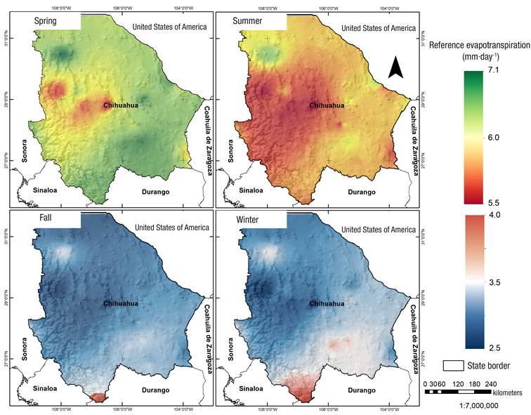
Figure 9 Spatial distribution of reference evapotranspiration (ETo) estimated by the Hargreaves method (1960-2013).
The seasonal analysis shows significant differences in the spatial distribution of ETo in Chihuahua, about the time of the year and altitude. On the other hand, for agricultural purposes, it is essential to represent the spatial distribution of the daily averages and annual cumulative values obtained with the Hg method. A standard deviation map of the annual ETo is also added to identify the areas with significant variability (Figure 10), which is helpful for water resource planning and management.
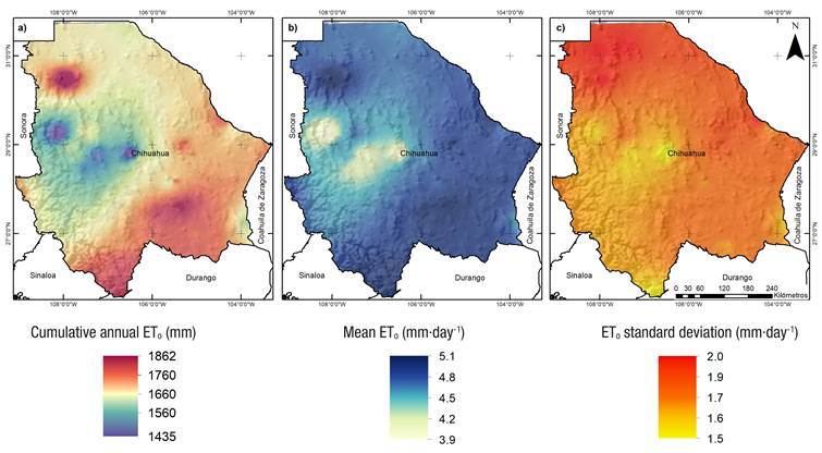
Figure 10 Spatial distribution of reference evapotranspiration (ETo) (a) annual cumulative (b) daily average, (c) standard deviation estimated with the Hargreaves method (period 1960-2013).
Monthly or annual cumulative ETo values are crucial for irrigated agriculture when a water balance is required to know the soil moisture content and determine periods of deficit or excess. Annual values ranged from 1 435 to 1 862 mm, while daily values ranged from 3.9 to 5.1 mm·day-1. These values are similar to those obtained by Orozco-Corral (2010) and Segura-Castruita and Ortiz-Solorio (2017).
Figures 10a and 10b show that the annual cumulative and daily average ETo values have similar spatial behavior. It can be observed that the minimum values are concentrated in the western and central regions (near the Peñitas and Majalca stations). A radial increase occurs towards the southern area (near the La Huerta station) and north (near the Dublan station) in the direction of the Sierra Madre Occidental. This behavior indicates that elevation plays an essential role in the distribution of ETo. An increase in height leads to a rise in ETo, especially in the warm seasons (spring-summer). It is because radiation is the primary energy source for ETo, as reported by Sun et al. (2020) and Tang et al. (2019).
The standard deviation is a measure of the dispersion of the data concerning the mean. In this sense, Figure 10c shows that the spatial variation of the daily mean values of ETo ranges between 1.5 and 2.0 mm·day-1 in the direction of the Sierra Madre Occidental. It confirms the effect of altitude on ETo estimation since it is observed that the higher elevations have lower variation compared with the great plains of the state had more significant variation during the period analyzed.
Conclusions
The empirical methods used underestimate ETo with significant differences concerning the reference method (PMMF). Besides, the methods that consider temperature as an input variable (Hg and Dg) are closer to PMMF, indicating that radiation is the primary energy source for the evapotranspiration process in arid and semi-arid areas.
On a monthly scale, the most significant differences between the methods compared occur in the warm months that coincide with the rainy season (June to September), and the methods closest to PMMF are Dg and Hg. The latter has the advantage of requiring only temperature measurements available at most meteorological stations in Chihuahua.
The spatial variation of ETo at the daily and monthly scales in Chihuahua directly relates to altitude, with maximums at low elevations and minimums at high peaks and is more evident in the warm months.
The IDW spatial interpolation method helps estimate the spatio-temporal variation of ETo over large extensions. However, in areas such as Chihuahua, where meteorological variables such as temperature and precipitation strongly influence ETo, it is recommended to try other spatial interpolation methods such as kriging or co-kriging, which have shown promising results with these variables.

