


 text in
  English (pdf)
 Article in xml format
 Article references
 Send this article by e-mail
 Cited by SciELO
  Similars in
SciELO
Similars in
SciELO 
 Permalink
Introduction
Hydrological phenomena are complex and difficult to understand, and in the absence of exact knowledge they can be represented in a simplified form by means of the system concept (Weber et al., 2012). A system can be understood as a set of elements or components related to each other by different processes (Rodríguez et al., 2006).
Due to the need to determine the effects of climate variation, climate change, land use changes and water resource management, several hydrological simulation models have been developed (Van Liew et al., 2005). The United States Department of Agriculture (USDA, 1986) mentions that hydrological studies should be based on historical flow records, but these are rarely available and statistical analysis becomes inaccurate due to land use changes. Therefore, Aparicio-Mijares (2008) indicates that it is necessary to have methods that estimate runoff from the characteristics of the watershed and precipitation, which are known as rainfall-runoff methods.
Although there are different programs for hydrologic modeling, Estrada-Sifontes and Pacheco-Moya (2012) mention that the Hydrologic Modeling System of the Hydrologic Engineering Center of the US Army Corps of Engineers (HEC-HMS) is a flexible program that allows selecting different methods for the calculation of losses, hydrographs, and river traffic; in addition, it allows simulating at the event level and on a continuous basis. Magaña-Hernández et al. (2013) predicted with HEC-HMS, the Escondido river watershed in Coahuila, with an area of 3 242 km2, for three hydrometeorological events, which are among the few with radar data (NEXRAD from NOAA of the USA) for hourly rainfall. These authors had almost perfect Nash-Sutcliffe coefficients (NSE), which was due to the fact that, at the time of calibrating the model, they left the range in which the hydrological parameters could move very flexible. The NSE measures the deviation with respect to the unit of the ratio between the mean square error and the variance of the observations (Singh, 2017).
In the hydrological region of the Fuerte River, Mexico, there is an important infrastructure for storing and supplying water for different uses, and for generating electricity and controlling floods. However, the incidence of extreme phenomena (such as hurricanes and droughts) is present, being unpredictable and with effects that can cause very serious economic damages (Comisión Nacional del Agua [ CONAGUA ], 2015).
Therefore, the objective of this paper was to build a calibrated and validated hydrological model, at hourly scale in subbasins belonging to the hydrological region of the Fuerte River, for extreme rainfall events of 2009, 2011, 2015, 2016 and 2017.
Materials and methods
Study area
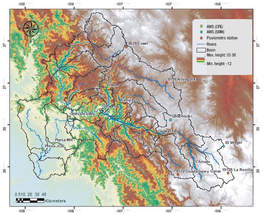
The hydrological subregion of the Fuerte River is located in northwestern Mexico, in the hydrological region number 10 of Sinaloa. Figure 1 shows how its surface area is distributed in Sinaloa, Chihuahua, Sonora, and Durango.
In the upper part of the watershed there are Tarahumara settlements, whose poverty levels are high, and in the lower part there are three dams (Miguel Hidalgo y Costilla, Luis Donaldo Colosio and Josefa Ortiz de Domínguez) for electricity generation and irrigation purposes (Castillo-Castillo et al., 2017). The dam system supplies water to two irrigation districts (RD): DR075 El Fuerte and DR076 El Carrizo, with a total area of 231 699 and 77 657 ha, respectively (CONAGUA, 2020). In addition, according to CONAGUA (2015), this subregion is exposed to the incidence of hurricanes in summer.
Once the available information on the watershed was reviewed, it was delimited with the HEC Geo-HMS 10.2 extension of ArcGis and based on the digital elevation model of the Instituto Nacional de Estadística, Geografía e Informática (INEGI, 2019a), up to station 25009 Bocatoma Sufragio of the Servicio Meteorológico Nacional (SMN, 2019a). With the same extension, the characteristics of the subbasins were obtained: slope, river length, lag time and HMS hydrological scheme (scheme or drawing with icons). The study area was delimited up to the Tubares station, which covers an area of 17 145.02 km2. The Huites, Miguel Hidalgo and Josefa Ortiz de Dominguez dams are outside the study area, immediately downstream of the Tubares hydrometric station. Tubares is in Chihuahua, approximately 39 km from the Huites Dam, Sinaloa.
Hydrometeorological information
Information from automatic weather stations (AWS) was provided by the Comisión Federal de Electricidad (CFE, 2019) and the SMN (2019b). The months reported were from June to October 2009, 2011, 2015, 2016 and 2017. Twenty-four h rainfall information was also requested from the SMN (Table 1). Figure 1 shows the location and spatial distribution of meteorological and hydrometric stations.
Table 1 Hydrometeorological stations in the upper watershed of the Fuerte River up to the Tubares station.
| Station | Administration/Type | State | Coordinate X, UTM (m) | Coordinate Y, UTM (m) | Information | Scale |
|---|---|---|---|---|---|---|
| Tubares | CFE/AWS | Chihuahua | 800062.98 | 2983759.21 | Flow Precipitation | 1 h |
| Urique | CFE/AWS | Chihuahua | 805824.31 | 3014204.43 | Flow Precipitation | 1 h |
| Batopilas | CFE/AWS | Chihuahua | 823729.33 | 2993087.05 | Flow Precipitation | 1 h |
| Guerachic | CFE/AWS | Chihuahua | 873443.76 | 2950383.58 | Flow Precipitation | 1 h |
| Urique | SMN/AWS | Chihuahua | 805386.86 | 3014070.40 | Precipitation | 10 min |
| Chinatu | SMN/AWS | Chihuahua | 922682.80 | 2907997.05 | Precipitation | 10 min |
| El Vergel | SMN/AWS | Chihuahua | 959766.68 | 2936360.79 | Precipitation | 10 min |
| Guachochi | SMN/AWS | Chihuahua | 890436.31 | 2971802.14 | Precipitation | 10 min |
| Maguarichi | SMN/AWS | Chihuahua | 795976.38 | 3085139.09 | Precipitation | 10 min |
| 8038 Creel | SMN/ Pluviometric | Chihuahua | 831477.88 | 3074041.35 | Precipitation | 24 h |
| 8106 Norogachi | SMN/ Pluviometric | Chihuahua | 883587.54 | 3024230.93 | Precipitation | 24 h |
| 8172 Guadalupe y Calvo | SMN/ Pluviometric | Chihuahua | 902646.84 | 2893908.09 | Precipitation | 24 h |
| 8266 Batovira | SMN/ Pluviometric | Chihuahua | 804700.54 | 3091986.56 | Precipitation | 24 h |
| 10125 La Rosilla | SMN/ Pluviometric | Durango | 966840.86 | 2898310.47 | Precipitation | 24 h |
CFE = Comisión Federal de Electricidad; AWS = automatic weather stations; SMN = Servicio Meteorológico Nacional; UTM = Transverse Mercator Coordinates.
Once the information was sorted and knowing that the series of hourly flow rates is continuous over time, the linear interpolation method was used to estimate the missing data, as long as there were no more than six continuous data. Gordon et al. (2004) mention that for short periods, linear interpolation can be used. For precipitation series, since they are not continuous (neither temporally nor spatially), the inverse of the square of the distance method was used.
Spatial and temporal distribution of precipitation for the hydrological model
The model was developed on an hourly scale, since the flow data measured by the CFE allowed it, taking into account that a large part of the watershed is operated by this institution, at least up to the dams where electric power is generated. It is important to clarify that the dams were located downstream of the calibration point (Tubares, Chihuahua) of the hydrological model.
Hourly rainfall data from eight automatic weather stations were used: four belonging to the CFE and four to the SMN. In addition, daily rainfall data from five SMN stations were used for a better spatial representation of rainfall in those areas that were not covered by the eight AWS. In the stations with cumulative rainfall values every 24 h, the proportional distribution of precipitation in the same period as the nearest AWS was used. This data management was used by Haberlandt et al. (2008).
To complete this part of the process, the spatial distribution of rainfall was determined using the Thiessen polygon method. The information on the predicted events is shown in Table 2.
Table 2 Hydrometeorological events selected for modeling the Fuerte river watershed.
| Storms | Start | Eind | Duration (days) | Maximum flow measured in Tubares (m3·s-1) | Total rainfall over the watershed (mm) |
|---|---|---|---|---|---|
| 2009 | 06/08/2009 08:00 | 30/08/2009 08:00 | 24 | 1 284 | 3 039 |
| 2011 | 18/08/2011 08:00 | 24/08/2011 08:00 | 6 | 296 | 504 |
| 2015 | 03/09/2015 08:00 | 18/09/2015 08:00 | 15 | 507 | 992 |
| 2016 | 16/07/2016 08:00 | 08/08/2016 08:00 | 23 | 935 | 2 074 |
| 2017 | 01/08/2017 09:00 | 09/08/2017 08:00 | 8 | 1 500 | 534 |
The World Meteorological Organization (WMO, 2018) considers that rainfall measurement at a given point only represents a limited area, which is bounded according to the accumulation period, physiographic homogeneity of the region, topography, and the different processes that favor precipitation. Espinosa-López et al. (2020) predicted the Huaynamota river watershed with hourly data from the CFE AWS and hourly satellite rainfall images. The model with AWS data gave better results in terms of fitting coefficient at the time of calibration and validation; therefore, data from the AWS were used in the present study.
Hydrologic modeling
Hydrologic modeling was performed using the HEC-HMS 4.2.1 program, with the U.S. Soil Conservation Service (SCS) method to transform rainfall into runoff, and the Clark unit hydrograph (U.S. Army Corps of Engineers [ USACE ], 2000) was used to calculate the hydrographs at the outflow of the subbasins. The modeling time interval was 1 h. The importance of building an hourly model lies in the relevance of using this model as a forecasting tool for civil protection purposes and to be more certain of the time when the highest flow will occur. It is also important to have an hourly model at those points in the watershed where the runoff concentration time is less than 24 h, since otherwise the model would not be useful for forecasting the time of the maximum flow. The calibrated model, in hourly terms, would be useful for decision making.
According to McCuen (2016), the equation for estimating the runoff is as follows:
where Q is the runoff or excess rainfall (mm), P is the precipitated rainfall (mm), S is the maximum retention potential of the watershed (mm) and I a is the initial abstraction (mm). Empirical evidence leads to the assumption that I a = 0.2S; considering this, Equation 1 is conditioned to P ≥ I a , otherwise Q = 0. Furthermore, the maximum retention potential is related to the curve number (CN) by the following equation:
According to USDA (1986), the runoff curve number is mainly a function of the hydrological group of the soil (A, B, C or D), type of cover and antecedent runoff condition. Curve number values were obtained from the same source for the different watershed conditions. CNA (1987) explains how to choose the hydrologic group according to the soil unit reported in the edaphological map of INEGI (2019b).
To calculate the runoff curve number, a curve number raster layer was first created using the vector data of soil type series II, and land use and vegetation series VI; both were downloaded from the INEGI digital platform (2019c). The curve number raster was performed in the HEC-GeoHMS extension, as indicated by USACE (2013) in the user manual of that extension. Once the curve numbers were calculated, the correction for slope was performed according to Neitsch et al. (2011):
where CN 2S is the curve number for condition II (CN 2 ) adjusted for slope, i.e., the condition when moisture content is considered average, and slp is the average slope of the watershed (%). USACE (2013) defines three antecedent moisture conditions: I dry (wilting point), II average moisture and III field capacity.
For each storm, the correction was made for antecedent rainfall accumulated five days before (Aparicio-Mijares, 2008) (Table 3). The conditions used for this purpose were: 1) correction A: when the antecedent rainfall is lower than 25 mm, 2) no correction: when the antecedent rainfall is greater than 25 and lower than 50 mm, and 3) correction B: when the antecedent rainfall is greater than 50 mm. A practical way to apply Equations 3 and 4 is shown in Table 3.
Table 3 Corrections of the curve number for antecedent moisture.
| No correction | Correction A | Correction B |
|---|---|---|
| 0 | 0 | 0 |
| 10 | 4 | 22 |
| 20 | 9 | 37 |
| 30 | 15 | 50 |
| 40 | 22 | 60 |
| 50 | 31 | 70 |
| 60 | 40 | 78 |
| 70 | 51 | 85 |
| 80 | 63 | 91 |
| 90 | 78 | 96 |
| 100 | 100 | 100 |
Source: Aparicio-Mijares (2008).
Synthetic unit hydrographs (SUH) can be used to calculate the maximum flow and runoff volume in a hydrograph, especially in ungauged watersheds. This study used the Clark unit hydrograph, which represents two processes of transformation of excess rainfall to runoff: 1) translation of excess rainfall from its origin through the drainage network to the outflow point and 2) attenuation of the amount of discharge once the excess is stored in the watershed (USACE, 2000). Straub et al. (2000) mention that flow attenuation can be represented as a linear reservoir, where storage is related to the outflow as follows:
where S is the storage in the watershed (m3), R is the storage coefficient (h) and O is the outflow (m3·s-1). From this relationship, the basic Clark unit hydrograph equation can be derived, where I is added as the inflow (m3·s-1) and C as the coefficient that is a function of the modeling step (h):
Hydrological models commonly use a time-related parameter, and the most used parameter is time of concentration (Campos-Aranda, 2010). Smith-Quintero and Velásquez-Henao (1995) indicate that the time of concentration is the time required for water to reach from the farthest point of the watershed to the exit point. Grimaldi et al. (2012) mention that, in practi/ce, empirical formulas are used to determine this parameter; one is that of Giandotti, which is highly used in Italy, another is that of Kirpich and that of NRCS, which are used in the USA. Table 4 shows different formulas to calculate this parameter.
Table 4 An overview of empirical and semi-empirical time-of-concentration estimation methods in hours.
| Method | Equation | Comments |
|---|---|---|
| Carter |
|
Developed for urban watersheds.Area lower than 20.72 km2Length of channels lower than 11.27 kmSignificant pipe flow in the watershedDeveloped from airport drainage data. |
| FAA |
|
Valid for small watersheds where laminar and overland flow dominate |
| Fórmula de onda cinemática |
|
Developed from the analysis of surface runoff kinematic waves |
| Kerby-Hathaway |
|
Area < 0.0404686 km2 Slope < 1 % n < 0.8 |
| Kirpich (Tenesee) |
|
Area of 0.00405 a 0.4532 km2 Slope from 3 to 10 % |
| US SCS |
|
For rural watersheds where overland  flow predominates Watershed area < 8.0937 km2 flow predominates Watershed area < 8.0937 km2
|
| Arizona DOT |
|
Modified form of FAAAgricultural watersheds |
| Giandotti-Fang |
|
Developed for small agricultural watersheds in Italy |
| California Culvert Practice |
|
Developed for small mountainous watersheds in California |
| Témez |
|
A = area (km2); C = runoff coefficient; CN = runoff curve number; E o = watershed outlet elevation (m); H = average watershed elevation (m); ΔH = difference in elevation between the start and end point of a channel (m); i = rainfall intensity (mm·h-1); L = length of the watershed along the main channel from the most hydraulically distant point to the outflow point (m); L c = length of the main channel (m); L ca = length measured from the concentration point along L to the point in L that is perpendicular to the watershed centroid (m); L’= Watercourse length (km); n = Manning's roughness coefficient; S = average watershed slope (m·m-1); Sc = average channel slope (m·m-1). Source: modified by Sharifi and Housenni (2011).
Using the HEC-GeoHMS extension, delay time can be calculated with the following expression (USACE, 2013):
Where Lag is the lag time (h), CN is the curve number, L is the hydraulic length of the watershed (m) and y is the average slope of the watershed (%). Hereafter, this method will be called SCS. It is important to remember that Lag = 0.6T c , where T c is the time of concentration. L is the length that corresponds to the time it takes for the water to travel from the hydraulically farthest point, this in terms of distance and slope, since water takes more time to reach the exit.
There are different studies that try to find the best formula to calculate the time of concentration, such as Sharifi and Hosseini (2011) and Vélez-Upegui and Botero-Gutiérrez (2011). The events with different times of concentration were predicted in this study, and the one with the best fitting coefficients in an initial modeling was chosen, specifically the one with higher NSE coefficients and lower root mean square error (RMSE) values for the same event.
Regarding the Clark unit hydrograph (Equation 5), the USACE (1967) recommends using a storage coefficient (R) with a value of 0.8 times the time of concentration. Zimmermann (2003) mentions that, in the absence of flow data, formulas such as R = cT c should be used, where c varies from 0.5 to 0.8. Magaña-Hernández et al. (2013) used a c of 0.75 when modeling a watershed in northern Mexico. This study used a value of 0.75 times the time of concentration.
Streamflow was determined using the Muskingum method (Equation 9). According to Karamouz et al. (2013), in that method the outflow hydrograph in the lower part of a river is calculated for a hydrograph determined in the upper part of the river.
where K is the travel time constant, and X is the weighting factor that varies from 0 to 1. According to Aparicio-Mijares (2008), K is equal to:
where L is the length of the section (m) and ꙍ is the wave velocity (m·s-1). Aparicio-Mijares (2008) mentions that K can be related as 1.5 times the mean water velocity in the channel. This study considered a reference velocity of 2.8 m·s-1, which is higher than the average velocity of natural channels not well defined on slopes of 12 to 15 % (2.4 m·s-1) according to Aparicio-Mijares (2008). The same author considers that, in the absence of information, it is recommended to use a value of 0.2 for the weighting factor. According to Heggen (1984), the value of X commonly varies from 0.2 to 0.3; therefore, the value used was 0.2.
Finally, a self-calibration was performed in the 2009 event, which allowed a maximum fit of 20 % in curve numbers, concentration times and, therefore, in the storage coefficient R. This was carried out with the optimization trial mechanism in HEC-HMS. Subsequently, validation was performed on the 2011, 2015, 2016 and 2017 events. Calibration and validation were carried out in three hydrometeorological stations of the CFE: Urique, Guerachic and Tubares; however, it was not successful in the first two (corresponding to runoff from subbasins of the upper part), so fitting in the Tubares station was considered as a reference. It is worth mentioning that the optimization trial mechanism follows the procedure shown in Figure 2, where the univariate gradient method was selected, and the objective function was evaluated with the NSE coefficient.
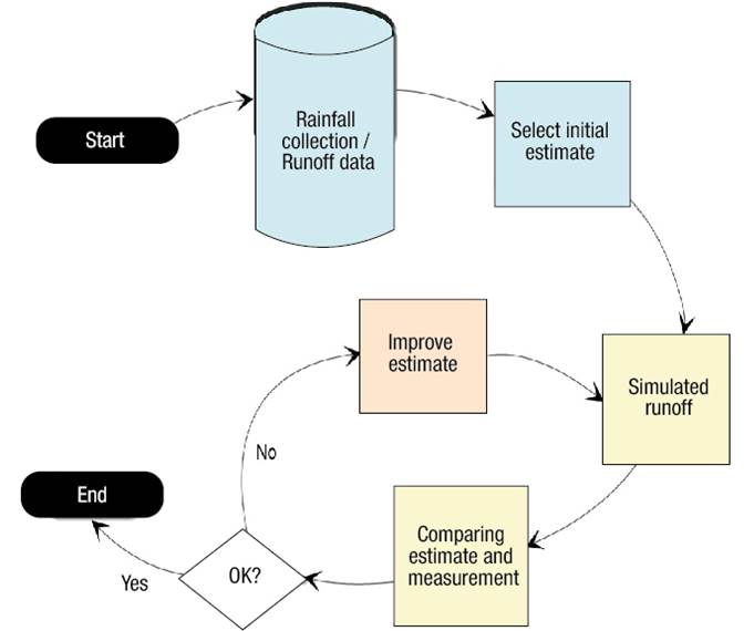
According to USACE (2000), the univariate gradient algorithm performs consecutive corrections to the estimated parameters. If x k is the parameter estimated by the objective function f(x k ) at iteration k, the search defines a new x k+1 at iteration k + 1 as:
where Δx k is the parameter correction and should be such that the estimates tend toward the minimum value of the objective function. The objective function can be the goodness-of-fit measured with the NSE coefficient, RMSE or others.
Goodness-of-fit of the hydrological model
The most used indicators to assess model fitting are NSE coefficient, RMSE, coefficient of determination (R 2 ) and mean squared error (MSE) (Vargas-Castañeda et al., 2015). The present study used NSE and RMSE. No reference of a good hourly hydrological model was found. Moriasi et al. (2007) present a general classification of recommended statistics to evaluate hydrological simulations with monthly step size, which is divided as follows: very good 0.75 < NSE ≤ 1, good 0.65 < NSE ≤ 0.75, satisfactory 0.50 < NSE ≤ 0.65 and unsatisfactory NSE ≤ 0.50. These authors also mention that values between 0 and 1 are considered acceptable levels of fit, since an NSE > 0 means that, at least, the model is a better predictor than simply using the arithmetic mean. Moriasi et al. (2007) show a general classification of recommended statistics for evaluating hydrologic simulations with monthly step size, which is divided as follows: very good 0.75 < NSE ≤ 1, good 0.65 < NSE ≤ 0.75, satisfactory 0.50 < NSE ≤ 0.65 and unsatisfactory NSE ≤ 0.50. These authors also mention that values between 0 and 1 are considered acceptable levels of fit, since an NSE > 0 means that, at least, the model is a better predictor than using the arithmetic mean.
Results and discussion
Figure 3 shows the subbasins corresponding to the modeling carried out, and their characteristics are shown in Table 5. The subbasins, up to the Tubares hydrometric station, have an average slope of 40.47 % and an average curve number of 79.04.

Table 5 Characteristics of the subbasins of the study area.
| Subbasin | Direct contribution to | Area (km2) | Slope (%) | CN2 | CN2S | Channel lenght (km) | Channel slope (m·m-1) |
|---|---|---|---|---|---|---|---|
| W1050 | Urique | 4 263.48 | 33.75 | 75.09 | 79.58 | 222.99 | 0.007 |
| W510 | Batopilas | 2 001.54 | 37.81 | 75.02 | 79.55 | 90.35 | 0.016 |
| W680 | Guerachic | 1 588.99 | 42.39 | 74.65 | 79.26 | 68.41 | 0.005 |
| W710 | Guerachic | 1 632.40 | 42.02 | 74.62 | 79.22 | 80.90 | 0.014 |
| W720 | Guerachic | 1 661.52 | 36.10 | 74.76 | 79.31 | 86.16 | 0.012 |
| W770 | Guerachic | 1 395.40 | 32.06 | 77.51 | 81.63 | 75.01 | 0.017 |
| W1250 | Guerachic | 42.57 | 62.11 | 77.54 | 81.76 | 2.93 | 0.009 |
| W1040 | Tubares | 423.17 | 58.32 | 72.11 | 77.07 | 53.57 | 0.005 |
| W840 | Tubares | 360.12 | 55.54 | 73.75 | 78.50 | 48.83 | 0.005 |
| W580 | Tubares | 356.40 | 47.58 | 72.18 | 77.12 | 28.95 | 0.002 |
| W610 | Tubares | 462.07 | 44.76 | 73.33 | 78.11 | 10.08 | 0.032 |
| W620 | Tubares | 588.85 | 50.76 | 67.98 | 73.42 | 32.68 | 0.001 |
| W640 | Tubares | 95.94 | 55.97 | 65.53 | 71.23 | 14.75 | 0.007 |
| W650 | Tubares | 1 195.16 | 48.14 | 72.62 | 77.51 | 57.77 | 0.008 |
| W660 | Tubares | 506.87 | 56.11 | 71.06 | 76.15 | 31.15 | 0.004 |
| W690 | Tubares | 396.43 | 46.47 | 78.68 | 82.71 | 58.64 | 0.000 |
| W1240 | Tubares | 161.21 | 53.98 | 74.02 | 78.72 | 19.62 | 0.008 |
| W900 | Tubares | 12.92 | 30.91 | 72.50 | 77.28 | 5.43 | 0.001 |
CN2 = curve number for condition II; CN2S = curve number for condition II fitted per slope
Concentration times calculated with different formulas are shown in Table 6. The maximum values are those calculated with the Giandotti and California Culvert formula, and the minimum values are those obtained with the SCS formula. Regarding the above, the events were predicted using these three times of concentration.
Table 6 Time of concentration, in hours, derived from different formulas.
| Subbasin | Giandotti | California Culverts | Kirpich | Témez | SCS |
|---|---|---|---|---|---|
| W1040 | 13.81 | 13.67 | 11.02 | 7.89 | 5.50 |
| W510 | 12.30 | 16.12 | 10.39 | 14.77 | 11.24 |
| W840 | 13.28 | 12.60 | 10.34 | 7.34 | 4.95 |
| W580 | 28.11 | 21.50 | 10.33 | 7.22 | 5.32 |
| W610 | 11.42 | 9.80 | 1.48 | 7.01 | 5.09 |
| W620 | 33.46 | 21.98 | 14.18 | 7.04 | 5.65 |
| W640 | 9.27 | 5.91 | 3.66 | 3.55 | 2.84 |
| W650 | 16.43 | 17.78 | 9.57 | 11.30 | 8.40 |
| W660 | 19.21 | 16.39 | 7.51 | 7.64 | 5.52 |
| W680 | 19.87 | 18.73 | 12.99 | 11.15 | 8.15 |
| W690 | 39.35 | 29.31 | 28.60 | 7.79 | 4.87 |
| W1240 | 9.21 | 6.08 | 4.27 | 4.09 | 2.68 |
| W710 | 12.28 | 14.88 | 10.09 | 12.87 | 9.52 |
| W720 | 14.44 | 19.41 | 11.32 | 15.35 | 11.96 |
| W770 | 11.29 | 14.58 | 8.84 | 13.77 | 10.28 |
| W900 | 18.16 | 7.75 | 3.92 | 2.12 | 1.66 |
| W1050 | 21.52 | 37.18 | 28.93 | 26.49 | 21.50 |
| W1250 | 12.11 | 6.43 | 0.94 | 2.64 | 1.48 |
SCS = Soil Conservation Service.
Table 7 shows the NSE coefficients derived from different concentration times. In 14 predicted events a better fit was obtained when the California Culvert method was used, three were better with SCS and two with Giandotti. The above coincides with the RMSE estimated, so the time of concentration calculated with the California Culvert Practice formula was used in this study.
Table 7 Nash-Sutcliffe coefficients calculated with the concentration times of Soil Conservation Service (SCS), California Culvert Practice and Giandotti.
| Event | Station | Nash-Sutcliffe coefficients | Best fit method | |||
|---|---|---|---|---|---|---|
| SCS | California | Giandotti | Maximum | |||
| 2009 | Tubares | -7.34 | -4.36 | -4.89 | -4.36 | California |
| 2011 | Tubares | -44.14 | -17.37 | -18.68 | -17.37 | California |
| 2015 | Tubares | -92.51 | -74.89 | -85.20 | -74.89 | California |
| 2016 | Tubares | -22.32 | -20.07 | -22.31 | -20.07 | California |
| 2017 | Tubares | -2.73 | -2.31 | -2.31 | -2.31 | California |
The values calculated in the 2009 event calibration are shown in Table 8, which were applied to each event and resulted in the curve numbers shown in Table 9.
Table 8 Calibration results for the 2009 event.
| Subbasin | Curve number | Time of concentration | Storage coefficient R (h) | |||
|---|---|---|---|---|---|---|
| Modification (%) | Value | Modification (%) | Value (h) | |||
| W1040 | -1.71 | * | -11.49 | 12.10 | 9.07 | |
| W1050 | 0.00 | * | -8.11 | 34.15 | 25.61 | |
| W1240 | 4.86 | * | -12.23 | 5.34 | 4.00 | |
| W1250 | 1.70 | * | 0.74 | 6.48 | 4.86 | |
| W510 | 14.87 | * | 6.25 | 17.12 | 12.84 | |
| W580 | 8.58 | * | -11.41 | 19.04 | 14.28 | |
| W610 | -1.28 | * | -8.50 | 8.96 | 6.72 | |
| W620 | 0.00 | * | -11.98 | 19.34 | 14.51 | |
| W640 | 0.00 | * | -10.79 | 5.28 | 3.96 | |
| W650 | -4.23 | * | -8.38 | 16.29 | 12.22 | |
| W660 | -1.76 | * | -9.98 | 14.75 | 11.06 | |
| W680 | 0.80 | * | -6.09 | 17.58 | 13.19 | |
| W690 | -2.31 | * | -9.63 | 26.48 | 19.86 | |
| W710 | -19.11 | * | -10.42 | 13.33 | 10.00 | |
| W720 | 0.00 | * | -8.78 | 17.70 | 13.27 | |
| W770 | -1.00 | * | -7.63 | 13.46 | 10.10 | |
| W840 | -0.01 | * | -8.01 | 11.59 | 8.69 | |
| W900 | 14.99 | * | 8.14 | 8.37 | 6.28 | |
*Variable value depending on antecedent rainfall (see Table 9).
Table 9 Curve number fitted for each event.
| Subbasin | 2009 | 2011 | 2015 | 2016 | 2017 |
|---|---|---|---|---|---|
| W1040 | 58.47 | 58.47 | 75.75 | 58.47 | 87.71 |
| W1050 | 62.49 | 62.49 | 62.49 | 62.49 | 79.58 |
| W1240 | 64.46 | 94.62 | 64.46 | 64.46 | 64.46 |
| W1250 | 66.75 | 93.44 | 66.75 | 66.75 | 66.75 |
| W510 | 71.74 | 91.37 | 71.74 | 71.74 | 91.37 |
| W580 | 64.65 | 64.65 | 64.65 | 64.65 | 83.73 |
| W610 | 59.96 | 77.11 | 59.96 | 59.96 | 77.11 |
| W620 | 55.11 | 55.11 | 73.42 | 55.11 | 73.42 |
| W640 | 52.47 | 71.22 | 52.47 | 52.47 | 71.22 |
| W650 | 57.47 | 85.72 | 57.47 | 57.47 | 74.23 |
| W660 | 57.35 | 87.13 | 57.35 | 57.35 | 57.35 |
| W680 | 62.61 | 79.89 | 62.61 | 62.61 | 62.61 |
| W690 | 65.52 | 90.22 | 65.52 | 65.52 | 65.52 |
| W710 | 50.21 | 64.08 | 50.21 | 50.21 | 64.08 |
| W720 | 79.31 | 62.17 | 62.17 | 62.17 | 90.58 |
| W770 | 64.79 | 64.79 | 64.79 | 64.79 | 64.79 |
| W840 | 61.20 | 78.50 | 61.20 | 61.20 | 78.50 |
| W900 | 68.69 | 68.69 | 88.86 | 88.86 | 88.86 |
Fittings on the curve numbers showed three cases: 1) decrease in eight subbasins (two of them runoff directly into the Guerachic station and the others directly into Tubares), 2) four subbasins had no changes and 3) two subbasins had direct runoff into Tubares, and there was increase in the Batopilas subbasin, in two subbasins of Guerachic and in three subbasins of Tubares. On average, the decrease was 1.76 % and the increase was 7.63 %.
With respect to time of concentration, an average decrease of 9.56 % was recorded in 15 of the 18 subbasins, and an increase of 5.04 % in three subbasins (Batopilas, one in Tubares and one in Guerachic), which represent 12 % of the total study area.
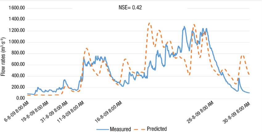
The NSE coefficients and RMSE for calibration and validations are shown in Table 10. Figures 4, 5, and 6 show three of the five predicted events. The results show an adequate fit at the Tubares station, with coefficients above zero. A negative value was obtained in the 2016 storm; however, the predicted hydrograph is temporally similar to that measured (Figure 6).
Table 10 Hydrologic model fit coefficients for the Fuerte River at the Tubares station.
| Coefficient | 2009 | 2011 | 2015 | 2016 | 2017 |
|---|---|---|---|---|---|
| NSE | 0.42 | 0.26 | 0.52 | -0.28 | 0.22 |
| RMSE (m3·s-1) | 248.13 | 58.28 | 74.03 | 243.84 | 337.08 |
NSE = Nash-Sutcliffe efficiency; RMSE = root mean square error.
Figure 4 Hydrograph of Tubares station, Chihuahua (August 2009 event).


The maximum flow rates measured and calculated are shown in Table 11. To contrast the visual interpretation (Figures 4, 5 and 6) and the model performance efficiencies (Table 10), Figures 7, 8, 9 and 10 show the behavior of that measured versus that predicted flow rates of the 2009, 2015, 2016 and 2017 events. Although the 2016 event had an NSE of -0.28, Figure 9 shows that the R2 is 0.59. This is important because if there were no error between that measured and predicted the trend of this relationship would be a straight line; therefore, the modeling of that 2016 event is not as negative as the NSE would suggest.
Table 11 Flows measured and predicted from the Tubares gauging station.
| Event | Hydrograph | Maximum flow (m3·s-1) |
|---|---|---|
| 2009 | Predicted | 1 282.50 |
| Measured | 1 283.70 | |
| 2011 | Predicted | 394.10 |
| Measured | 296.00 | |
| 2015 | Predicted | 402.50 |
| Measured | 506.50 | |
| 2016 | Predicted | 1 387.10 |
| Measured | 934.80 | |
| 2017 | Predicted | 853.90 |
| Measured | 1 499.90 |
Figures 7, 8, 9 and 10 show the goodness-of-fit for three hydrometeorological events from 2009, 2015, 2016 and 2017, respectively.
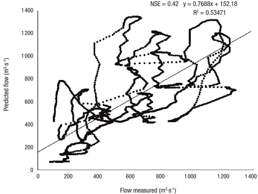
Figure 7 Goodness of fit between that measured and predicted in the August 2009 event in the upper Rio Fuerte watershed.
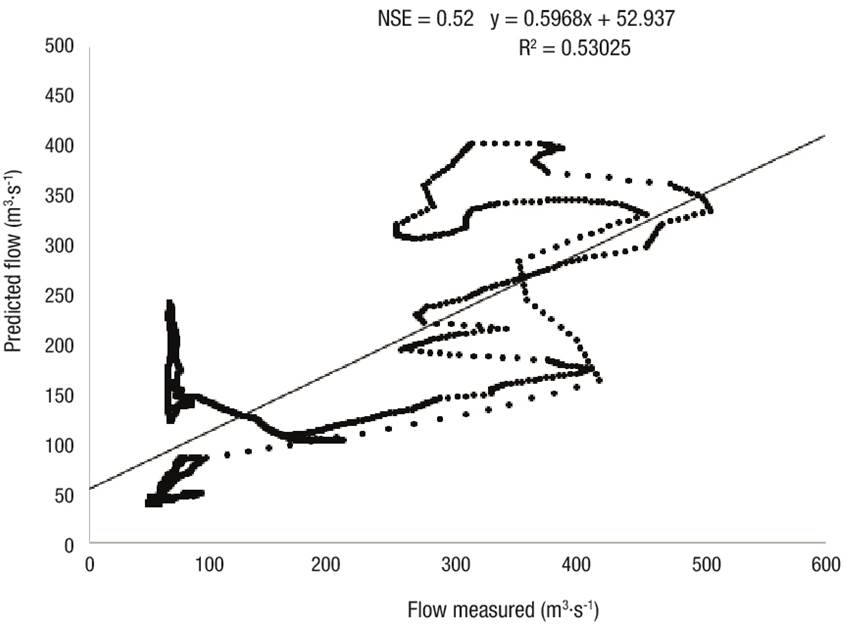
Figure 8 Goodness of fit between that measured and predicted in the September 2015 event in the upper Rio Fuerte watershed.
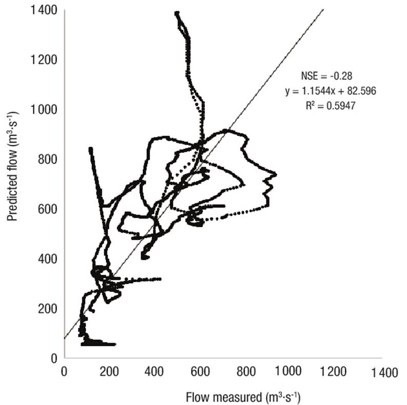
Figure 9 Goodness of fit between that measured and predicted in the July/August 2016 event in the upper Rio Fuerte watershed.
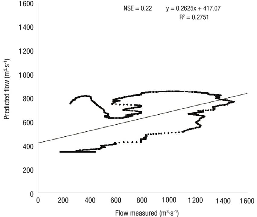
Figure 10 Goodness of fit between that measured and predicted in the August 2017 event in the upper Fuerte River watershed.
The model fit would be expected to have a relationship with the maximum flow measured; however, the results show no influence. For example, in the calibration of the 2009 event, an NSE coefficient of 0.42 was obtained for a maximum discharge measured of 1 283.70 m3·s-1 (Figure 7), while the 2015 validation had an NSE of 0.52, corresponding to a maximum flow measured of 506.50 m3·s-1 (60.54 % lower) (Figure 8), and the 2017 event, with a flow of 1 499.90 m3·s-1 (16.84 % higher), had an NSE of 0.22 (Figure 10). Moriasi et al. (2007) consider, for a calibration and validation on a daily scale, a value greater than 0.4 as satisfactory.
If we compare the NSE of 0.4 of this study with the 0.95 of the hourly hydrological model of Magaña-Hernández et al. (2013), for the Escondido river watershed, Coahuila, it would seem that this study is at a disadvantage. However, in the Escondido river model, too much correction margin was given to the hydrological parameters at the time of calibration. That is, the hydrological parameters were allowed to vary up to any value and at any level of increase or decrease, regardless of the reality of their values, which gave them an almost perfect model. Another aspect is that in that study they had some radar images of rainfall provided by the USA due to the proximity to Texas. It is convenient to improve the hourly hydrological modeling due to its importance in civil protection and in those points where the time of concentration of the watershed is less than 24 h. However, modeling should be done preserving the principles of the modeler representing the reality it intends to simulate.
The visual analysis of the Tubares station shows temporal similarity between the predicted and measured hydrographs. Considering the coefficients obtained, it can be said that the model found at the outlet of the Tubares subbasin represents, at an acceptable level (Moriassi, et al, 2007), the hydrometeorological phenomenon in the study area, because it shows a satisfactory fit in calibration and in one of the validations.
An attempt was also made to calibrate the model at two upstream hydrometric stations but was unsuccessful. One possible explanation is that rainfall varies more spatially in mountain areas. Moreover, WMO (1972) recommends one station per 100 to 250 km2 for mountainous areas, and in the study watershed there are 14 stations (eight AWS and four pluviometric stations with daily data) distributed over 17 145 km2; that is, one station covers an average of 1 224.64 km2, which leads us to think that rainfall may not be well represented in this area.
On the other hand, good fitting at the outlet is attributed to two aspects: 1) the transit of the flow from the upstream stations until reaching the outlet and 2) the contributions of 11 subbasins (lower part), which are not calibrated individually (as is the case of the upstream subbasins Urique and Batopilas), but up to the Tubares station, which allows compensating the bad fitting caused by the contributions of the upstream subbasins.
Haberlandt et al. (2008) mention that simple hydrological models provide an objective global estimate, but at the cost of smoothing the hydrograph, which leads to underestimation or overestimation; this is observed in the hydrographs measured in the present study. Perhaps this model could be improved by considering a distributed model that uses information from satellite images of hourly rainfall and that is calibrated with data from the CFE. Another improvement to the model would be to generate measured unit hydrographs, instead of the synthetic Clark unit hydrographs used in this study.
Although one might believe that it is not worthwhile to build hourly hydrological models in Mexico because there is not enough measured rainfall and hourly flow data, it is important to prepare for the future and strive to develop a sufficient and reliable hydro-meteorological network.
Conclusions
The hydrologic model developed at the outlet of the Tubares watershed using the curve number method to calculate losses and Clark's synthetic unit hydrograph method for hydrographs, is acceptable based on the Nash-Sutcliffe coefficients.
The time of concentration that yielded the best modeling results is the one calculated with the California Culvert Practice formula, which overestimates the correct value by about 10 %. An alternative to improve modeling could be the use of an aggregated model that uses information from satellite or radar images to estimate rainfall. It is also recommended to model individually the upper subbasins with different methods than those used in the present study, for example, a different unit hydrograph or a different spatial distribution of rainfall. All this to obtain a general model that properly represents hydrology in the entire watershed.

