


 text in
  English (pdf)
 Article in xml format
 Article references
 Send this article by e-mail
 Cited by SciELO
  Similars in
SciELO
Similars in
SciELO 
 Permalink
Introduction
A culvert is defined as a short passageway or closed conduit to transport water from one place to another, usually on transport routes (road, rail or other embankment), which in turn contributes to meeting the needs of surface drainage, thus fulfilling the function of a passage structure for water and protection for transport routes (Chaudhry, 20008; Schall, Thompson, Zerges, Kilgore, & Morris, 2012). When the culvert inlet is submerged, its operation corresponds to an orifice (American Society of Civil Engineers/Water Environment Federation [ASCE], 1992; Normann, Houghtalen, & Johnson, 1985; Urban Drainage and Flood Control District [UDFCD], 2016) or a gate (Henderson, 1966); otherwise, its behavior is similar to the flow of a broad-crested weir (ASCE, 1992). If the outlet is submerged, it is called a drowned discharge or, failing that, a free discharge (Normann et al., 1985; Tullis & Robinson, 2008).
In hydraulics, knowing the behavior of structures during their operation is essential; for this, it is necessary to determine, experimentally, the relationship between the variables of interest, which is called the characteristic curve. In particular, for control structures (such as orifices, gates, weirs, siphons, among others) a relationship between the operating load and the discharge is sought (Charbeneau, Henderson, & Sherman, 2006). In a culvert, two types of control can be presented: 1) inlet, in which the discharge that can pass through the conduit depends only on the conditions of the inlet, and 2) outlet, in which the characteristics of the conduit and the outlet must be added together (Alonso, 2005).
Traditionally, analysis of submerged and unsubmerged inlet operation is done separately, resulting in curves that may or may not overlap; this makes identification of the transition uncertain (Charbeneau et al., 2006). Huffman, Fangmeier, Elliot, and Workman (2013) show a composite curve for weir and orifice operation without considering this zone.
Until the middle of the last century, the transition zone was given little importance and was not considered in hydraulic culvert design procedures (Charbeneau et al., 2006). At the end of the last century, Normann et al. (1985) proposed a simple operating curve for culverts, in which they indicated the operating curve of the orifice and the weir with a tangent line joining both curves. Likewise, Charbeneau et al. (2006) started from the individual curves and made a least-squares fitting for the transition zone. Considering that there is not enough information about the hydraulic behavior in a weir-orifice transition in culverts, and with the hypothesis that the behavior of the load-flow ratio is not linear, the aim of the present work was to obtain the characteristic curve of the real behavior of the transition zone of a culvert with inlet control, as well as the mathematical models of the hydraulic operation. This was done by varying the water level continuously in a physical model designed, built and instrumented with low-cost sensors.
Materials and methods
Culvert design
The design of a culvert requires a local hydrological study to obtain the design discharge (Chanson, 2000). Typically, storm-produced runoff is assumed to have a return time of 25 to 50 years (Alonso, 2005). The design discharge and embankment height are associated to determine the diameter or height of the conduit, or conduits, as the case may be. The minimum diameter of the conduit is 0.31 m (12”) for culverts in channels (Arteaga, 1992), and from 0.40 to 0.60 m for relief ones (García-Trisolini, 2011). The Colombian Ministerio de Obras Públicas (MOP, 1967) recommends a minimum diameter of 0.91 m (36 in) for major roads considering their required maintenance work, and 1.22 m (48 in) or 1.52 m (60 in) for those areas where there is considerable sediment drag. Likewise, on secondary roads the diameter should not be less than 0.61 m (24 in), nor less than 0.46 m (18 in) on roads or access routes according to the Nicaraguan Ministro de Transporte e Infraestructura (MTI, 2008), which mainly considers maintenance. The conduit’s cross section depends on the height of the embankment, construction cost, material and type of inlet (Chanson, 2000; Clark & Kehler, 2011; Schall et al., 2012).
Regarding length, the variable to be examined corresponds to the width of the obstacle to be crossed. According to the Secretaría de Comunicaciones y Transportes (SCT, 1991), for safety reasons, the minimum lane width is 4 m to be able to travel at 60 km·h-1, in addition to one-meter clearance on each side for pedestrian movement, which generates a width of 6 m for a single-lane road and 10 m for a two-lane one. The operating speed must be between 1.5 and 2.5 m·s-1 to meet the demands of load losses and silting (Arteaga, 1992), although the MOP (1967) specifies that the permissible speed depends on the physical characteristics of the terrain.
Finally, the construction slope, a parameter that directly governs the drainage capacity of the work, for a culvert in channels may have a zero slope (Arteaga, 1992); however, Schall et al. (2012) recommend a minimum slope of 0.005 % to ensure good drainage. For a relief culvert, there are no restrictions because it depends directly on the relief conditions present at the site; however, Arteaga (1992) mentions that the location should comply with certain characteristics that regulate the water speed and avoid damage to the hydraulic work. The MTI (2008) establishes that the culvert’s longitudinal slope should not be less than 1 % to avoid silting up, but it must respect the permissible speed. Another factor to consider is the functional aspect or non-hydraulic functions, such as the passage of fish (Clark & Kehler, 2011).
Design and construction of the culvert-type hydraulic model
The work was carried out at the hydraulics laboratory of Chapingo Autonomous University’s Irrigation Department. A real culvert or a much-used culvert was taken as an example, with a water speed of 1.5 m·s-1, a conduit diameter (D) of 0.53 m (21 in), a zero slope and a length (L) of 6 m. These characteristics meet the design specifications for culverts. Using the Froude similarity law, commonly referred to as Bernoulli's principle for real flow, the model scale was obtained (with the continuity and energy equation), and the geometric and hydraulic characteristics of the model were designed. Table 1 presents the values obtained in the calculation of the equations used, and Figure 1 shows the conceptual model for the construction of the hydraulic model.
Table 1 Values calculated with the Froude similarity law for the culvert-type hydraulic model.
| Dmz (inch) | Dm (m) | Le | Qe | Ve | Vm (m·s-1) | Qm (m3·s-1) | Qm (L·s-1) | Lm (m) | Ɛ/D | Re | f |
|---|---|---|---|---|---|---|---|---|---|---|---|
| 1.76 | 0.0448 | 11.9 | 489.145 | 3.45 | 0.43 | 0.0007 | 0.685 | 0.50 | 3.35x10⁻⁵ | 1.93x10⁴ | 0.026 |
zDm = model diameter; Le = line scale; Qe = flow scale; Ve = speed scale; Vm = speed in the model; Qm = model flow; Lm = model length; Ɛ/D = roughness/diameter ratio; Re = Reynolds number; f = energy loss factor.

The hydraulic model consists of two acrylic-based containers and a 0.05 m (2 in) tube bonded with glue. The upstream container with dimensions of 0.42 x 0.35 x 0.35 m has a perforated plate 0.09 m away from the wall, in front of the conduit inlet to stabilize the flow, and the downstream container is 0.37 x 0.35 x 0.35 m and has an 8 cm diameter perforation in the center of the bottom for release purposes. In addition, the system has PVC pipes of 0.05 m (2 in) in diameter, with an arrangement for the support of the model, in order to guarantee the autonomy of the system and to facilitate the operation and transport. The device was powered by two motor pumps (an Evans® brand model 1HME025 and an Siemens brand model 1RF21000FA404EB1) by means of pipes, union nuts, elbows and a gate valve at each outlet to vary the inlet flows of 0.025 m (1 in) and PVC suction piping of 0.032 m (1 1/4 in) in diameter. Likewise, to ensure water circulation, a drainage system was made and installed based on PVC piping that leads to a 0.11 m3 (110 L) container.
Physical model instrumentation and sensor calibration
The second stage of model construction corresponded to the instrumentation of the device. For this, a plate (Arduino Uno®), an ultrasonic distance sensor (HC-SR04) and a flow meter (FS400a water flow sensor) were used.
The flow meter was located in the model's feeding area. For its calibration, the relationship between the number of blade revolutions (pulses) and the discharge was determined, for which a code was made in Arduino to record an average every five cycles. The discharge was obtained by the volumetric method using a 1 L graduated cylinder for small flows and 5.35 and 10.54 L containers for larger flows; time was measured with two stopwatches. The results obtained were fitted to a linear of the form y = a + bx with Equations1 to 5, reaching a coefficient of determination (R2) of 0.998 (Infante-Gil & Zarate-de Lara, 1990). The calibration curve is shown in Figure 2.
Where NP corresponds to the number of pulses, Q to the discharge (L·min-1), SPNPQ is the covariance, and SPQ and SPNP are the variances.

The ultrasonic distance sensor was calibrated by testing to find its operating accuracy, and an average error of 0.0012 m and a standard deviation of 0.003 m were obtained, which ensured the reliability of the readings. This sensor was installed at a distance of 0.15 m upstream of the culvert inlet, and at a height of 0.35 m from the bottom of the container, measuring the distance to the free water surface.
Figure 3 shows the physical model to measure the culvert operating variables, in which the feeding, control and measurement parts are indicated.

Taking readings and debugging data
With the sensors calibrated and installed in the physical model, the process consisted of setting up the feeding system and taking readings of water surface heights and flow with variations in the inlet discharge by means of gate valves. Due to the existence of extreme data caused by hydraulic transients during the valve opening, it was necessary to debug with an Arduino Uno® code specifically designed to rule out cycles where the data will show differences greater than or equal to two pulses for discharge measurement, or a discrepancy of 0.001 m in the distance sensor. The debugged data were fitted to a model of the form Q = k·h m for the domains delimited for weir and orifice. Equations 6 and 7 were used to obtain the parameters k and m, and Equations 8 to 11 the determination coefficient.
Where h is the operating load (cm), n is the number of data and SC h is the sum of squares.
The transition zone was fitted to a linear model with the equations described in the calibration of the FS400a flow sensor, for which the operating load in cm was set in “x” and the discharge in L·m-1 in “y”.
Results and discussion
Operation of the culvert-type hydraulic model
With the data obtained, the curve shown in Figure 4 was drawn, where the orifice, weir and transition type hydraulic operating intervals are highlighted.
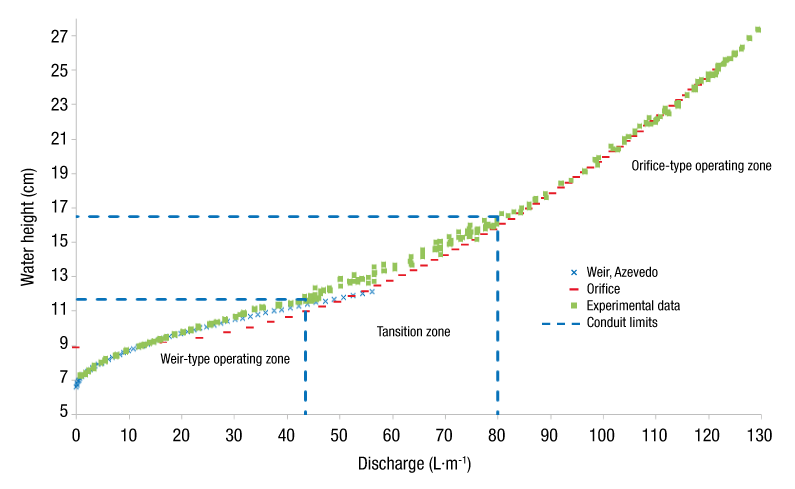
With the different zones identified, delimited and fitted to a mathematical model, Equation 12 was obtained. The zone corresponding to the circular weir (Figure 5) was fitted to a potential model, which had an R2 of 0.99 due to the incidence of an undular hydraulic jump caused by the depression of the inflow at the point of change from weir to orifice, or from canal to short pipe (Figure 6), which provided differences in the upper operating limit; however, when compared with the equation proposed by Azevedo-Netto and Acosta-Álvarez (1976), concordance between the two curves can be seen.
Where, for the studied model, Q is the discharge (L·min-1), and h v , h t and h o are the pressure load (cm) on the weir, transition and orifice, respectively; their origin is the center of gravity of the piping. All cases in Figures 4, 5 and 9 represent the values of a circular culvert of the model or prototype where the conduit coincides with the base of the canal and the height of the water above the orifice is not measured at the center of gravity of the piping, but from the bottom of the conduit.

Figure 5 Water height-discharge curves: experimental vs. theoretical data on the weir-type operating zone. D = conduit diameter (m); h = operating load (cm).

Figures 7 and 8 show the model operating as an orifice with free discharge at the culvert outlet. The fit had a potential model Q = 28.521·h 0.5201 with an R2 of 0.997. The root function (exponent m = 0.5), commonly used to evaluate orifices Q = Cd·A(2g·h) 0.5 , gives us a discharge coefficient (Cd) of 0.75 and has a maximum difference of 2.2 % between the equation fitted with k = 28.521 and m = 0.5201, and the equation with Cd = 0.75 and m = 0.5. Considering a height of 0.111 m in the conduit key, the minimum height for it to work as an orifice is 0.167 m to guarantee compliance with the specification of 1.2 times the diameter, which ensures an orifice-type hydraulic operation.

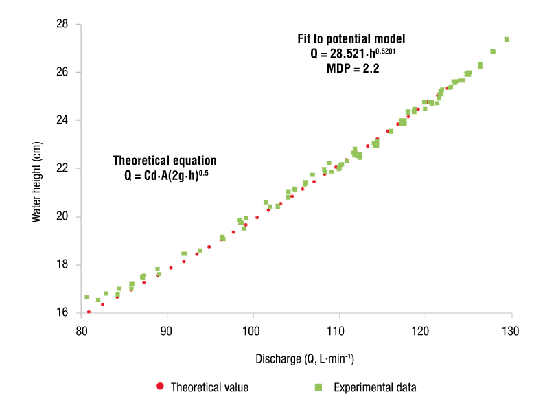
Figure 8 Water height-discharge curve: experimental vs. theoretical data on orifice-type operation. MDP = maximum percentage difference; Cd = discharge coefficient; A = orifice area (m2); g = gravity (9.81 m·s-2); h = operating load (cm).
Figure 9 shows in greater detail the section between the heights 0.117 to 0.165 m, corresponding to the transition zone; that is, when changing from weir to orifice operation, the points are scattered due to the lack of load at the limit where it stops functioning as an orifice (Figure 10). Under the previous condition, the conduit is partially filled with undulations caused by the flow depression (Figure 11). Therefore, the transition was fitted to a quadratic model, which differs from what was observed by Charbeneau et al. (2006), Normann et al. (1985) and Schall et al. (2012), who present the weir and orifice curves as a straight line; however, their simplification is acceptable, since only 0.2 % accuracy is lost and its operation is easier.


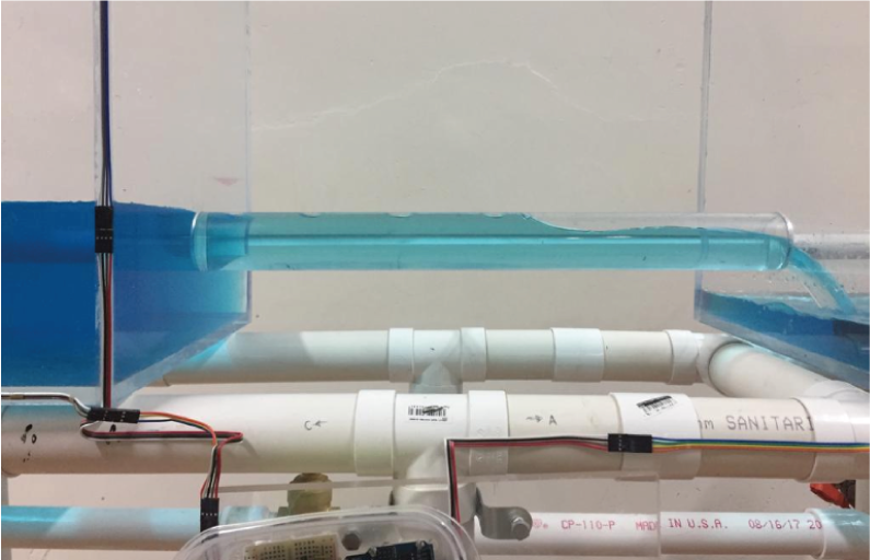
Figure 11 Flow in the partially-filled conduit when the culvert operates in the weir-orifice transition zone.
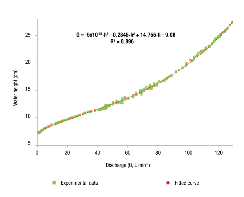
Finally, by using a function that integrates all the above equations in the range of 0.066 to 0.29 m (Figure 12) to simplify the model, the following equation is obtained:
with a coefficient of determination of 0.996; that is, the discharge prediction would have an error of less than 1 %. It is important to emphasize that using this general third-order polynomial expression eliminates the function of the transition zone, since the fit does not distinguish the different types of hydraulic operation.
Conclusions
According to the design, construction, installation, instrumentation and operating characteristics of the system, it was a success; however, it is recommended to experiment with different conduit diameters to avoid problems of scale in the results transferred to the prototypes. The FS400a and HC-SR04 sensors yielded reliable results compared to those measured in the development of this research. The global model Q = f(H) ranged from 0.066 to 0.286 m; 25 % of the water surface heights (0.066 < H ≤ 0.117 m) behaved as a weir, 23.53 % (0.117 < H ≤ 0.165 m) corresponded to the transition zone and 51.47 % (0.165 < H ≤ 0.286 m) behaved as an orifice. For the section operating as an orifice, a Cd of 0.75 was determined for a circular shape. It was found that if the operating load does not have 1.2 times its diameter, it does not behave as an orifice. The weir and orifice zones were fitted to a model of the shape Q = k·h m with an R2 of 0.992 and 0.997, respectively.
Considering the orifice and weir operations separately, and joining them with a tangent line, does not provide a good estimate of the actual behavior in the structure since the transition zone begins when the load is less than 1.2 times the diameter. In reality, the weir-orifice transition exhibits a curved trend, not linear as stated by several authors. With the simplification to a linear model, the results in practice are acceptable since only 0.2 % accuracy is lost. Finally, the hydraulic operation of the culvert can be described by Equation 13; however, it is important to emphasize that using this general third-order polynomial expression eliminates the transition zone, since the fit does not distinguish the various types of behavior.

