


 text in
  English (pdf)
 Article in xml format
 Article references
 Send this article by e-mail
 Cited by SciELO
  Similars in
SciELO
Similars in
SciELO 
 Permalink
Introduction
The irregular distribution and uncertainty of water resources, as well as the need to produce food in Mexico, has led to the opening of large irrigated areas in arid and semi-arid regions (Ojeda-Bustamante, Hernández-Barrios, & Sánchez-Cohén, 2008), since approximately 50 % of national agricultural production comes from irrigated areas (Ojeda-Bustamante et al., 2008). Most of the infrastructure built in Mexico's irrigation districts was sized under the criteria of the former Secretaría de Recursos Hidráulicos (SRH, 1973). The design method traditionally used to determine the capacity of canals was proposed by that Ministry; however, in other countries, different methods are used that generate more efficiency (Íñiguez-Covarrubias, de León-Mojarro, Prado-Hernández, & Rendón-Pimentel, 2007; Íñiguez-Covarrubias, Ojeda-Bustamante, & Rojano-Aguilar, 2011). It should be noted that, in recent years, the Irrigation District (ID) Management division of Mexico's Comisión Nacional del Agua (CONAGUA) has conducted several studies in the IDs called "Master Plans," in order to determine the need for and plan investments (Instituto Mexicano de Tecnología del Agua [IMTA], 2007).
The dominant water distribution method in Mexico’s irrigation areas is by weekly controlled demand, and consists of planning the volume of water withdrawal from the supply source by the distribution network for delivery to users within a period of seven days, this according to the irrigation requests received from users in the previous week (Arista-Cortes, González-Camacho, & Ojeda-Bustamante, 2009). According to the classification of distribution methods, the responsibility for controlling the distribution of dominant irrigation in Mexico is shared (User-Authority [CONAGUA]), and is known as controlled demand (Íñiguez-Covarrubias et al., 2007).
In the irrigation service delivery process, the average efficiencies of the water distribution system must be known. These efficiencies should be considered when planning water allocation. Consequently, it is vital to implement robust irrigation scheduling schemes, preferably in "near real time," to achieve efficient use of resources and operate, hydraulically, the canal network satisfactorily (Spare, Wang, & Hagan, 1980).
To obtain the reference evapotranspiration (ETo) of the crop, in order to determine the capacity of the canal, it is recommended that irrigation area designers estimate it based on robust methods such as the Penman-Monteith method modified by FAO (Allen, Pereira, Raes, & Smith, 2006), as well as use the concept of growing degree days (°D), since it is an adequate tool to predict the phenology and development of the crops, which will help to better adjust the irrigation supply to the water needs of crops. Íñiguez-Covarrubias et al. (2011) used this methodology to determine canal capacity. To do this, they estimated evapotranspiration in an irrigation area (ETia) in five steps. Additionally, it is important to consider that the calculation of irrigation depths corresponds to the useful storage capacity of the soil within the root depth (SRH, 1973).
Currently, with the innovation and application of computer tools, which facilitate the handling of large volumes of information on different useful variables, it is possible to perform laborious numerical calculations. An example of this is the estimation of the irrigation requirements that are important to match the water demands of the crops with the application of irrigation through the hydraulic infrastructure (Ojeda-Bustamante, Sifuentes-Ibarra, Íñiguez-Covarrubias, & Montero-Martínez, 2011). However, the current conservative idea of operation limits the natural evolution of irrigation areas and the updated information of the variables of interest, which prevents improving the service and generates large water losses due to deficient operation in periods of peak irrigation demand (Íñiguez-Covarrubias et al., 2007, 2011).
Today, one of the main challenges for researchers related to the management of large irrigation areas, divided into several irrigation modules or sections, is to efficiently perform the calculations and generate accurate and timely recommendations. With this, there is no doubt that large irrigation systems can be designed and operated more efficiently (Ojeda-Bustamante, Sifuentes-Ibarra, & Unland-Weiss, 2006; Ojeda-Bustamante et al., 2008).
Based on the bibliographical review carried out for the development of this paper, and on the works carried out by the authors in several IDs, for the Irrigation User’s Civil Associations (ACURs), the ACUR federations called SRLs and CONAGUA, it is known that there is no explicit, integrated procedure to implement hydrosystemic management with application in complex irrigation systems that have different crops, varieties, soils, planting dates and agricultural seasons. A Mexican ID may have one or more SRLs, which are responsible for executing the works and activities that are common to two or more ACURs.
Therefore, the objective of this work was to propose and analyze a function in which three variables converge: crop evapotranspiration (ET), water distribution planning, and canal capacity. Subsequently, the aim was to develop a proposal for hydrosystemic management in which the variables are combined with the greatest degree of flexibility to satisfy the user and meet the expectations for the use of water resources. To this end, it is important to consider the agronomic, soil and climatic conditions and the type of irrigation infrastructure.
Materials and methods
Study area
The study was conducted in the “Santa Rosa”, module which is part of the ID-075, located in Valle del Fuerte, Sinaloa, Mexico. In this region, the rainy season is concentrated mainly in the months of September and October, often of cyclonic origin. The evaluated irrigation module covers an area of 34 316 ha, has a crop repetition factor in the spring-summer (S-S) season of up to 27 % and stands out as the largest module of ID-075.
The procedure for the allocation of irrigation (delivery-receipt) in the “Santa Rosa” module is based on a weekly irrigation schedule. The operation of the headworks (storage dam) is the responsibility of the federal authority (CONAGUA). Irrigation frequency is scheduled in each ACUR and the duration is agreed upon by the User-ACUR binomial. The delivered flow is limited by the farm's intake capacity (120 L·s-1 on average). With these operating conditions, the irrigation module reports an overall annual operating efficiency of 51.4 %, a value that reflects the water distribution method used in ID-075.
It is important to point out that in ID-075 there is a culture of systematization of agricultural and hydrometric information. The "Santa Rosa" module has a very complete database with information from the last 17 agricultural years, which has been generated with the "Spriter" real-time irrigation forecast system developed by Ojeda-Bustamante (1999). The historical weather information used corresponds to the monthly average values of the 1961-1990 period of the “Los Mochis” weather station, located in the center of the irrigation district. Because the study area is in a semi-arid region, precipitation was not considered, since the period of maximum irrigation demand occurs in the dry periods of the year.
Crop plan
The standard irrigation plan of the irrigated area was considered, which includes planting dates and areas per crop. The most important crops in ID-075 are corn, sorghum, bean, fruit trees, sugar cane, fodder (mainly alfalfa) and vegetables (tomato and potato). The net depths were considered at the farm intake level (where ACUR delivers water to the users) and the gross is at the control point level (where ACUR receives water from the ID's SRL).
Crop water demands were established for annual planning purposes. For this, data were taken from the study conducted by Mendoza-Robles and Macías-Cervantes (2003) on corn, one of the main crops of the "Santa Rosa" module. These authors indicate the optimal planting date in relation to the probable yield loss in final production (kg·ha-1), as well as the planting date, season length (days), ETo (mm), potential evapotranspiration (ETp) (mm) and number of irrigations.
The determination of canal hydraulic capacity was carried out using the Clement method (Íñiguez-Covarrubias et al., 2011). For design purposes, farm application efficiency (η) was 70 % for gravity irrigation, as well as for conduction and distribution in earth-lined canals (SRH, 1973). The overall efficiency for design is estimated as ηoverall = ηconduction x ηapplication, which is 49 % for the earthen canals, as reported for the “Emilio Grivel” canal. In addition, for serving large cultivated areas, the time of the irrigation service is considered to be 24 hours a day.
The development of the methodological proposal for hydrosystemic management is summarized in the following six stages:
Stage 1. The ETo is estimated and the ETp is calculated by crop and planting date. The concept of accumulation of °D is used as an alternate criterion to express the duration of the phenological cycle of crops and thus estimate the crop coefficient based on the °D according to the equations of Ojeda-Bustamante et al. (2006 and 2008). In this case, an ETp curve is constructed for each planting date, which integrates the planting period, in the irrigation area. The ETp of a crop (assumed as the maximum ET without water, nutritional, thermal or phytosanitary stress problems), from the planting date (PD) to the harvest date (HD), is given by the following equation:
where
To estimate the ETp, the historical climatology and a cropping plan that includes the proposed crops with dates, planting areas and agricultural season are required. Since rainfall during the period of peak demand is minimal in Mexico’s irrigation districts, it is assumed that the ET is equivalent to the crop's irrigation requirements. In the case where effective precipitation is important during a crop’s period of peak demand, it should be subtracted from the daily ET. For more information on the methodology used, consult the work of Íñiguez-Covarrubias et al. (2011).
Stage 2. Irrigation is scheduled for each planting date of each crop. To determine the irrigation depth, it is necessary to know the type of soil, bulk density, field capacity, permanent wilting point, depth of the roots of the crops (for different stages of development) and the irrigation practice used for each crop.
Stage 3. Based on the results of applying Equation 1, the cumulative ET curve (ETc) is constructed for each crop, which will be referred to as ET1c to indicate an integrated curve of several planting dates of a crop in an agricultural season: autumn-winter (A-W), spring-summer (S-S) and perennial crops. Irrigations are specified according to each crop, until obtaining the ET1c in cm for the established multicrop area. At this stage, partial results are obtained for the number of hectares established, irrigation schedules, and the flow required to satisfy demand is compared with the flow available in the canal for each delivery point. Ojeda-Bustamante and Flores-Velázquez (2015) point out that ETc ≈ ETp for minimum stress conditions. It should be noted that, for each day i, ET 1C = f j x ET c-i , where fj is the weight of each planting date j (Íñiguez-Covarrubias et al., 2011).
Stage 4. At this stage, the unique curve of hectares established for the crop (in this case corn) per season is constructed, which is composed of the hectares of the different planting dates. It should begin with the first ten days of the agricultural year (in this case on Julian day 281), until reaching the total planting of the crop; the cropping area per planting date is taken into account. In this part of the process, the number of hectares with scheduled irrigations for each ten-day period (irrigated hectares) is obtained.
Stage 5. The area and the ET are integrated for each agricultural season (ETseason), considering the per-crop occupation of each season (S-S, A-W and perennial). In this way, the ETseason, the quantity and the specific location of hectares with irrigations scheduled for each ten days are partially obtained, which facilitates the estimation of the necessary and available flow in the canal at the specific water delivery points.
Stage 6. The joint general function of the three seasons (S-S, A-W, and perennial) for the agricultural year is obtained, thus obtaining the area variable with the total irrigation requirement in the zone and for ten-day periods. The information matrix obtained based on Table 1 has n columns. The filling in of the matrix begins in column n(i=1), season and the initial day (Julian day: Day), which is from the planting date per crop until the last day of the phenological stage. The “Crop” column is filled with the result in tabular form of the ETp per day for each planting date of stage 1, the area (number of hectares) and, finally, the corresponding irrigation dates for the crop. Column n(i=2) is for crop 2, and the filling in is repeated as in column n(i=1), only that the results are placed as the beginning on the subsequent days that separate the planting from the beginning of crop 1. In this way, column n(i=3) is for crop 3, and the filling in is repeated as in columns n(i=1) and n(i=2), placed on the Julian days subsequent to the Julian start of the planting date of crop n, and so on until all the crops are completed with their planting dates of the A-W, S-S and perennial seasons. There will be as many columns n(i) as the number of crop planting dates. Each line of column 6(a) lists the area with crop every day of the year, which is the sum of the areas of each crop by planting date, and column 6(b) lists the areas per ten days with irrigation, at the end of each day of the ten.
Table 1 Functional matrix that integrates the participation of each planting ten-day period for a crop per season.
| 1 | 2 | 3 | 4 | 5 | 6 | 7 | ||||
|---|---|---|---|---|---|---|---|---|---|---|
| Day | Crop n(i=1) | Crop n(i=2) | Crop n(i=3) | Crop n(i=2) | Area (ha) | Volume demanded (1 000 m3) | ||||
|
|
Area (A) (ha) | Irrigation date (I) | ETp, A, I | …. | … | (a) | (b) | (a) | (b) | |
| Established | Ten-day irrigation | Daily | Ten-day period | |||||||
The complete matrix provides the number of hectares with water requirement, the irrigation depths, which when multiplied by the hectares yields the daily ten-day volume (includes total efficiencies), and the flow needed to satisfy the water demand with the available flow in the distribution canal for each delivery point. As can be seen, at this stage the irrigation demand, irrigation distribution planning, and hydraulic capacity of the canals are integrated into a joint function.
Due to the large number of calculations involved, the algorithms for estimating the ET of the crops in an irrigation area, according to the methodology proposed by Íñiguez-Covarrubias et al. (2011), were coded in Java language, in a program developed by the authors called IntegraRR, based on the CROPWAT program (Clarke, Smith, & El-Askari, 1998), but which uses the concept of growing degree days. This program was also used to integrate the functional matrix in Table 1 for each crop, by season and by agricultural year.
Results and discussion
The results are presented on the basis of the development of the six stages of the methodological proposal for hydrosystemic management. In this way, the ETo was estimated and the ETp per crop and the planting date were obtained according to Equation 1. Figures 1 and 2 show the distribution of the cropped area established per Julian day (%) for each crop in the A-W and S-S seasons, respectively, in ID-075 (IMTA, 2007). In the curve of each crop, the planting date considered to generate the curves is indicated with a dot.
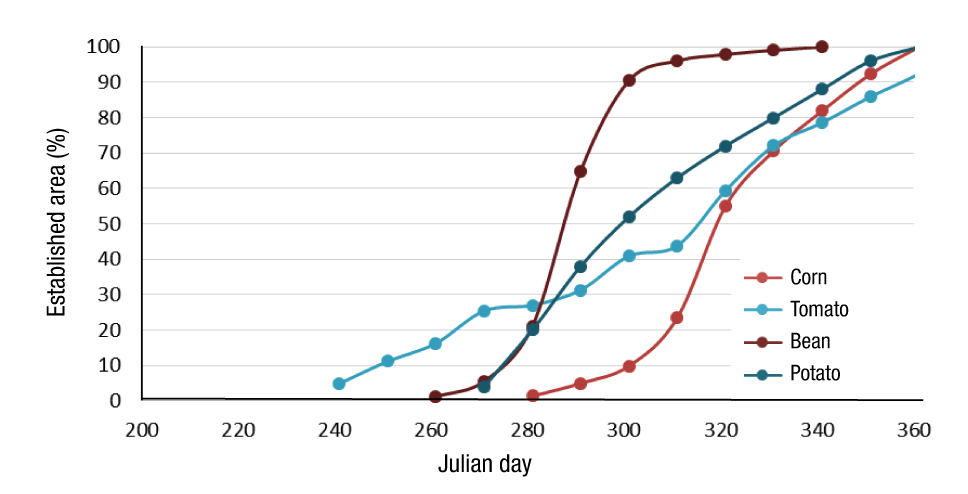
Figure 1 Distribution of planting dates in the autumn-winter season. Source: Author-made with data from the Mexican Institute of Water Technology (IMTA, 2007).
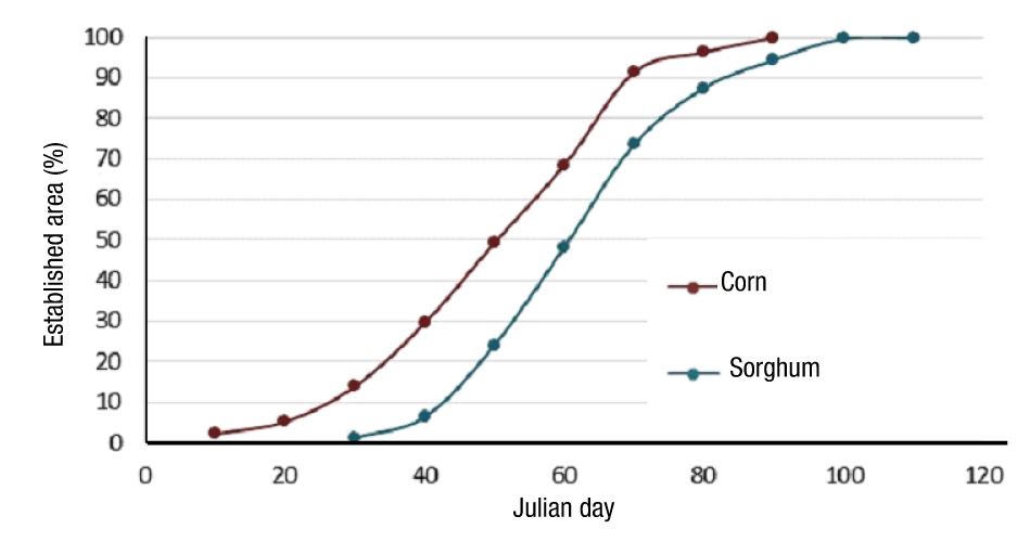
Figure 2 Distribution of planting dates in the spring-summer season. Source: Author-made with data from the Mexican Institute of Water Technology (IMTA, 2007).
The irrigation depths are applied per crop according to the irrigation policy and where the number of irrigations is variable, since the following irrigation is applied when the maximum allowed water depletion is consumed according to the crop and the phenological stage. The net depth applied to the crops is of the order of 10 cm for relief irrigation, except for tomato, which requires a net depth of the order of 8 cm. For its part, the gross depth is affected by the efficiency reported by the “Santa Rosa” module for the A-W, S-S and perennial seasons.
Figure 1 shows that the planting period for corn is from the first days of October to the end of December, for bean from the end of September to mid-November, for potato from the end of September to the end of December and for tomato from the beginning of September to the end of December. In addition, it can be seen that the tomato crop does not have any period with all the established area, as it has a long planting period, so the first harvests are presented in the overall planting period considered. In the case of bean, potato and corn, planting ends before the first harvests, so they have a period where the established area is 100 %.
Since corn is the most representative crop in the area, the results of applying Equation 1 are shown for this crop (stage 1). Figure 3 shows the daily ETp curve of corn for a planting date (Julian day 350, ten-day planting 8), in which five irrigations with accumulated ETp of 50.62 cm were supplied. The area established in the ten days was 1 135.51 ha, which represented 10.4 % of the corn planting in the A-W season.
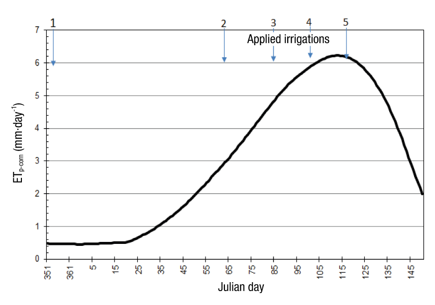
Figure 3 Daily potential evapotranspiration (ETp) of corn for the 10-day planting date 8 (December 16, 2004) with five irrigations.
The irrigation distribution system in this proposal is a ten-day period; the first irrigation takes place on day 1, and subsequent irrigations on days 67, 87, 107 and 125. The irrigation depth is 10 cm per event and the minimum irrigation interval is 17 days. The canal flow is 1.87 m3·s-1, which is necessary due to the conditions of the canal with 49 % efficiency.
Figure 4 (stage 4) shows the curve of the established cumulative area of corn for the A-W season, as well as the irrigation hectares for the ten-day periods, starting with the first period on Julian day 281 until reaching the last period to have a total established area of 10 918 ha. The maximum volume required for corn in the A-W season was estimated at 557 134.56 m³·day-1, which is demanded on Julian day 99 (April 9, 2005), corresponding to the maximum ET1c of 5.3 mm·day-1 and an established area of 10 383.36 ha (Figure 4). The programmed ten-day area is 7 129.8 ha, with a design capacity flow in the canal of 8.18 m3·s-1, required flow of 8.17 m3·s-1 and a 16-day interval, this for a weekly irrigation distribution system with delivery on Monday or Thursday, and overall efficiency of 63 %. By increasing conduction efficiency from 70 to 90 %, a 10-day interval is achieved.
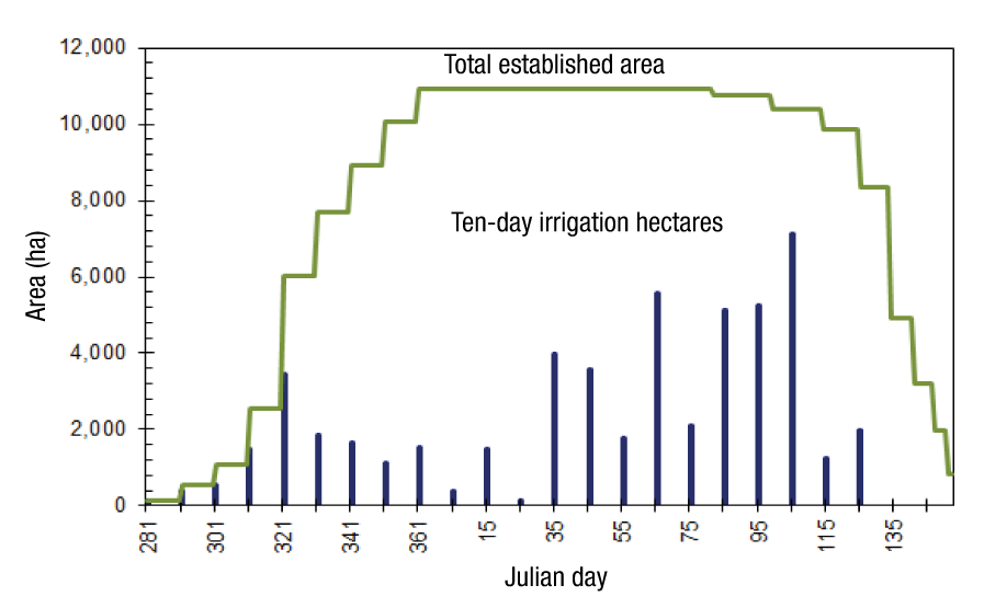
Figure 4 Total established area and ten-day irrigation hectares for corn in the autumn-winter season.
Figure 5 shows the process of integrating ET curves, first by planting dates for a crop (ET1C), then by agricultural season (ETseason), which corresponds to the ET of each season analyzed (ETA-W, ETS-S and ETPER), and finally the integrated curve for the irrigation zone (ETIZ) (Íñiguez-Covarrubias et al., 2011).
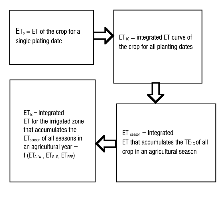
Figure 5 Integration process of evapotranspiration (ET) from a planting until its integration by crop, season and irrigation area.
Figure 6 (corresponding to stage 5) integrates the ET 1C-i curves of all the crops in the A-W season to obtain the ETA-W. The values for the A-W season are highlighted with the peak volume required for Julian day 105 (April 15, 2005), with a maximum volume demanded of 672 200.7 m3·day-1, ETA-W of 5.172 mm·day-1, area of 11 643.0 ha established (potato with 1 051.33 ha, corn with 10 383.36 ha and tomato with 208.42 ha), 10-day programmed area of 7 416.8 ha, capacity flow in the canal of 8.18 m3·s-1, required flow of 8.17 m3·s-1 and a 16-day interval, this for a weekly irrigation distribution with delivery on Monday or Thursday, and an overall efficiency of 63 %. In this case, the capacity of the entire canal is already available; that is, there is no capacity restriction.

Finally, upon completion of the methodology proposed in stage 6, the integrated general matrix of the three seasons (S-S, A-W and perennial) for the agricultural year is obtained. Figure 7 shows the relationship of the hectares established for each day for the entire irrigation area, in addition to the hectares with 10-day irrigation requirements for all ten-day periods of the year. The highest value occurs on Julian day 105 (April 15, 2005), with a maximum volume of 918 487.63 (m3·day-1), peak ETIZ of 4.07892 mm·day-1 and an area of 22 518.0 ha established. For the ten days from 105 to 115, with an overall design efficiency of 51.3 %, a flow of 21.70 m3·s-1. would be required.
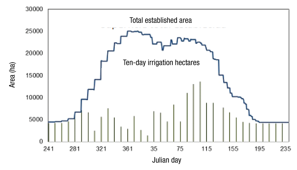
Figure 7 Total established area and ten-day irrigation hectares for the three agricultural seasons (autumn-winter, spring-summer and perennial).
The ten-day period with maximum demand on the irrigation system is from Julian day 101 to 111 (April 11 to 21, 2005), with an area of 13 548 ha, of which 1 985 ha are of the S-S season, 7 416 ha of the A-W season and 4 146 ha of the perennial season. Here again, the full capacity of the canal is available, so there are no restrictions and the flow of 27.185 m3·s-1 is available. The flow in the design of the canal with Clement's method is 27.86 m3·s-1, which is greater than the flow required for the maximum ten-day period.
With respect to the planned irrigation volume to be used under the crop plan, ACUR reports a gross planned volume (without efficiency at the control point at the beginning of the module) of 226 480 thousand m3, and the volume estimated by integrating the curve in Figure 7 is 154 544.00 thousand m3, which is 47 % less than that the irrigation volume planned for delivery to the users. The above is a real indicator of the overall efficiency of the hydrosystem, that is, of the ID under the hydrosystem management proposal.
Conclusions
The ten-day systematization of crop water demand facilitates knowledge of the area associated with the irrigation requirement from the beginning of the first planting of each crop and for each season until the last irrigation demanded in an irrigation area. With the temporal knowledge of the hectares with irrigation requirements, the weekly distribution of water through the network is adjusted; it also estimates the required daily flow to apply for all seasons, this when knowing the date and required irrigation in the ten-day period.
In this case, it is concluded that the capacity of the canal, in any irrigation section, is not a limitation for applying the irrigation plan. This implies that for any other irrigation plan, the proposed hydrosystemic management methodology would have to be repeated, in which the three main variables of the large irrigation areas concur; that is, the water demand of the crops, the water distribution planning and the determination of the hydraulic capacity of the canals.
Regarding the irrigation service, it can be said that full user satisfaction depends solely on the proper management of the Irrigation User’s Association, since for the infrastructure and for the conditions of the irrigation plan there are no limitations as long as the irrigations are programmed, on the basis of a mutual agreement between the Authorities and Users.
Based on the results obtained, implementing a hydrosystemic management system, such as the one proposed herein, is widely recommended for any ID, according to the technological advances in computing, measurement, communication and control. Therefore, support programs and trained personnel are required for water management in complex, large-scale irrigation systems with different crops, planting dates, types of irrigation application systems, agricultural seasons and different irrigation modules or sections.

