


 text in
  English (pdf)
 Article in xml format
 Article references
 Send this article by e-mail
 Cited by SciELO
  Similars in
SciELO
Similars in
SciELO 
 Permalink
Introduction
In applications where heat transfer must occur only at particular locations, it is necessary to design an efficient water distribution system. At those locations, a device such as a heat exchanger (HE) will transfer heat via conduction or thermal radiation. A number of studies have evaluated specific heating and cooling systems with respect to their ability to solve their heating, ventilation and air conditioning (HVAC) problems, using distributed pipe systems. Bobenhausen (1994), Castro, Song, and Pinto (2000) and Sugarman (2000) found that such systems might lose a considerable amount of heat as the transport fluid circulates through the system. Meanwhile, Picón-Núñez, Polley, Canizalez-Davalos, and Medina-Flores (2011), Ponce-Ortega, Serna-González, and Jiménez-Gutiérrez (2010), and Sanaye, Mahmoudimehr, and Aynechi (2012) looked at the impact of distributed cooling and heating systems dealing with variables such as heat loss, pressure drop, system capacity and system optimization. In special cases, the complex phenomena involved in heat transfer were analyzed through alternative methods, such as Artificial Neural Networks and optimization schemes (Barteczko-Hibbert, Gillot, & Kendall, 2009; Hosoz, Ertunc, & Bulgurcu, 2007).
Choi, Cook, and Nordlund (2014), Mondaca, Rojano, Choi, and Gebremedhin (2013) and Ortiz et al. (2015) pointed to the need to develop a hydraulic and heat transfer modeling tool for a large-scale, distributed conductive cooling system to mitigate heat stress in dairy cows. Bastian, Gebremedhin, and Scott (2003) presented the concept of a HE applied to a conductive cooling system for dairy cows. Mondaca et al. (2013) further developed a comprehensive model that analyzed such HE. Later, Choi et al. (2014) proposed an enhanced HE and Perano, Usack, Angenent, and Gebremedhin (2015) experimentally evaluated a HE to reduce risks related to lame cows (Cook & Nordlund, 2009). Most recently, there has been interest in connecting each HE to warrant the practicality of designing and building a large-scale, cold-water distribution system.
Therefore, the aim of this work was to propose a water supply system connected to a series of HEs, installed under bedding in a dairy barn freestall system, to cool down cows exposed to heat stress and analyze heat transfer along a large-scale water pipe network. For this purpose, EPANET software version 2 (United States Environmental Protection Agency ENT#091;US EPAENT#093;, 2008) was used as the platform for the code development, since this program enables simulating a pipe network and calculating heat transfer rates. Given that every real-world application requires a particular pipe network design and operation, the aim of this work was to lay down the foundation for a generalized solution, one that can be used to produce a viable hydraulic model.
EPANET is dedicated to developing large-scale systems (potable water, fire protection, and field irrigation). More specifically, researchers have used the program to compute the hydraulic parameters that determine the characteristics of a system’s key components, such as pipes, various fittings, reservoirs, water sources, valves, and pumps (Andrade, Kang, Choi, & Lansey, 2013; US EPA, 2008). It is hypothesized that EPANET can also be effectively used to calculate the heat transfer rates of large-scale heating and cooling systems based on a heat and mass transfer analogy (Incropera, DeWtt, Bergman, & Lavine, 2011).
Materials and methods
This investigation proposes a methodology for handling hydraulics coupled with heat transfer of a water distribution system. For simplicity the entire system was divided into two sections, one containing all the HEs and the other being the Water Supply System (WSS). EPANET software was used to analyze the WSS as a hydraulic model in order to determine the most feasible characteristics of the pipe network and the best operating conditions. In addition, the EPANET module called Water Quality Solver (WQS) was used. This module is used for chlorine concentration and decay in municipal water distribution systems, to modify the mass balance component of the model and turn it into a heat balance model using the heat and mass transfer analogy.
Efficiency of the WSS must be evaluated with respect to whether it is gaining or losing heat along the way with different heat transfer rates at each HE, and the total energy needed to operate it. To simulate hydraulic performance and total pumping power of the system in EPANET software, parameters such as pipe network layout, flow rate demanded by each HE, spatial distribution of HEs and pipe characteristics (length and diameter) must be included. Thus, a hydraulic model’s thermal performance can be set by defining thermal properties of the pipes and insulation (pipe material, inside pipe wall roughness, pipe wall thickness and its thermal conductivity) in conjunction with corresponding thermal boundary conditions (temperature or heat fluxes in the boundaries). Finally, the range of operation will be defined by combining parameters that determine hydraulic and thermal performance. From these conditions, a set of numerical solutions can be found and used to determine which hydraulic and thermo-physical parameters will conveniently increase the system’s efficiency.
Figure 1 shows the process followed in designing the pipe network supplying water at each HE. First, the pipe network layout and its characteristics must be established in order to find the hydraulic parameters within an achievable range of operation. These data will determine the simulated network’s pumping requirements and parameters for heat transfer rates. Second, it is necessary to include settings for the pipe’s thermal boundary conditions that, combined with dimensionless parameters for heat transfer, will compute changes in water temperature and, consequently, the system’s cooling capacity. In the present study, the values representing water’s thermo-physical properties, such as viscosity, density, and the Prandtl number, remain constant based on the average operating temperature.
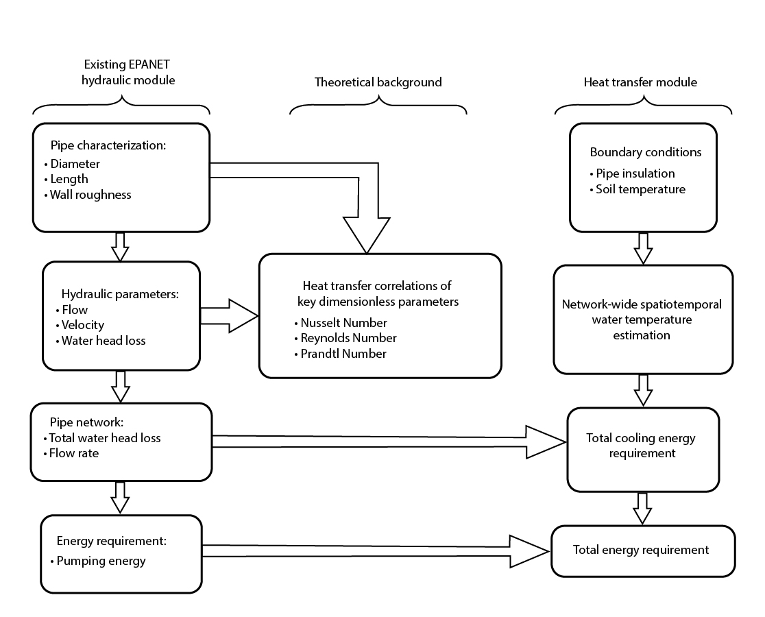
Figure 1 Flowchart to develop a heat transfer module in conjunction with existing EPANET hydraulic module.
Hydraulic model
Pipe network design determines the hydraulic model in terms of the flow rates, velocities and pressure drops occurring in each pipe. The American Water Works Association (AWWA, 2004) recommends that water velocities in water distribution systems should be below 3 m·s-1. Also, to make sure that water passes through the entire loop, EPANET computes the total water pressure and flow rate needed. The simulation must include information regarding minor losses occurring locally (based on what types of junctions are used), and so the appropriate coefficients required based on the recommendations of the US EPA (2008). For this investigation, the flow rate was defined by the HE demand.
Layout of the WSS was considered to be composed of three sectors: 1) the pipes that delivered and returned water to the HEs, 2) the elements that represented the HEs, and 3) the flow control valves that ensured same flow rates would occur in each HE. Pipes delivering and returning water followed a similar path. Elements representing HEs connected both sections by means of pipes that were equivalent in length and water volume.
Heat transfer solver
The heat transfer rates were defined by the thermal boundary conditions, either by assuming that the heat flux or the temperature remained constant. No matter which one was assumed, conditions can be uniform within any single pipe. In this case, all heat transfer calculations were based on a constant temperature. To quantify heat flow changes, the heat transfer solver should run according to the hydraulic model.
Heat transfer rates, primarily estimated by applying analytical equations about convection and conduction, can be governed by how well the system was operated, type of pipe, thermal properties of insulation, flow regime, thermal boundary layer, and environmental conditions involved. In the convection section, water flow regime is subjected to laminar, transitional or turbulent conditions, each of which can influence heat transfer rates differently. Rates of conductive heat transfer depend on thermo-physical properties of materials for pipes and insulation, considering also data of inside wall area and roughness of pipes.
Heat carried by water running through the pipe network can be quantified by applying advection equation (Equation 1), which can simultaneously find the heat gained or lost along the pipe wall as water moves. EPANET’s hydraulic model can simulate water movement, and it can be used to find parameters required to conduct a thermal analysis of such variables as flow rates and water velocities.
Since many applications imply setting non-uniform thermal boundary conditions, the proposed heat transfer solver is capable of dealing with constant parameters at each pipe, such as thickness of the pipe wall and insulation (along with their corresponding thermal conductivity values). A constant temperature can be assumed on external walls of each pipe or insulation (T epw ) and at both ends of each pipe (T wi and T wo ), and every pipe wall can be assumed uniform in its thickness, and thickness of its corresponding insulation (dy). A summary of heat transfer is shown in Figure 2a and parameters for conductive cooling in Figure 2b.
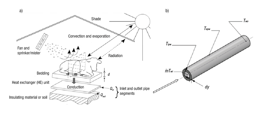
Figure 2 a) A schematic of a conductive cooling heat exchanger for dairy cattle (Mondaca et al., 2013) and b) variables involved in heat exchange associated with a pipe.
Advection model
The advection equation was used to estimate temperature variation using the Lagrangian approach:
where T i is temperature in pipe i (°C), t is time (s), x is location within the pipe (m), u i is axial velocity in pipe i (m·s-1), and S i is temperature change per second due to wall heat transfer at pipe i (°C).
Temperature at junctions
Pipe junctions caused flows to mix, and affected the corresponding water’s temperature. At any junction, some pipes supplied water, and other pipes conducted water into the rest of the network. Assuming that perfect and instantaneous mixing occurred at all junctions, temperature at any junction can be calculated:
where i denotes the pipe leaving junction k, I k is the set of pipes that supply flow into junction k, L j is length of pipe j (m), and Q j is flow in pipe j (m3·s-1). Notation T i|x=0 represents temperature at the beginning of pipe i (°C), while T j|x=Lj is temperature at the end of the pipe (°C).
Constant temperature is assumed at the pipe’s external wall insulator. Since insulation is not perfect, the interior wall tenperature changed, modifiying the water temperature, which produced a water temperature gradient between the beginning and end of each pipe:
where T i,wi is water temperature at the beginning of the pipe (°C), and T i,wo is water temperature at the end of pipe i (°C); the latter can be determined by the following expression:
where T i,ipw is pipe wall interior temperature (°C), P is pipe perimeter (m), L is pipe length (m), h is heat transfer coefficient (W·m-2·°C-1), ṁ i is flow for pipe i (kg·s-1), and Cp is specific heat (for water: 4 182 J·kg-1·°C-1). To calculate the h with a water flow regime under transitional or turbulent conditions, we used the following equation (Gnielinski, 1976):
where k f is water thermal conductivity (W·m-1·°C-1), Re i is Reynolds number for pipe i, Pr is Prandtl number (equal to 7.01), and f i is friction factor; the latter can be calculated using the Colebrook-White equation:
where e is roughness height (m), and D i is diameter of pipe i (m). This equation applies to turbulent conditions (Re > 4 000). The f i , in laminar flow regime can be computed by:
The Equation 5 is acceptable under transitional and turbulent conditions, with the following conditions: 0.6 ≤ Pr ≤ 2 000 and 2 300 ≤ Re ≤ 106. Margin of error increases within a transitional flow regime, and it becomes higher once it nears the laminar flow regime. Nonetheless, Equation 5 uses the uniform wall temperature approach, where its error can be considered negligible according to Abraham, Sparrow, and Tong (2009).
Equations 6a and 6b are designed to cover laminar and turbulent conditions; however, the equation for finding f i for transitional flow regime is not well defined. Therefore, EPANET computes f i by cubic interpolation taken from the Moody diagram based on the Reynolds number (US EPA, 2008). With respect to heat transfer, if the flow regime is within laminar conditions, then heat transfer coefficient can be calculated by:
Because pipe segments can be partially insulated, external wall temperature will cause heat to be exchanged at a rate defined by the pipe wall’s thermal properties. The internal pipe wall temperature (T i,ipw ) can be found by solving for equilibrium between convection and conduction:
where q cond is heat by conduction (W), q conv is heat flow by convection (W), k p is thermal conductivity of pipe or insulation (W·m-1·°C-1), A i is pipe wall surface area (m2), dy i is pipe wall thickness (m), T pwe is external pipe or insulation wall temperature (°C), and ṁ is mass flow (kg·s-1). In cases where more than one layer of insulation exists, the overall thermal conductivity was computed in series, along with their corresponding thicknesses. Substituting Equations 9 and 10 into Equation 8, value of T i,ipw - T i,wo can be obtained and substituted into Equation 4 to solve it for T i,ipw , and then find the water temperature at the end of the pipe (T i,wo ).
Heat exchanger
Depending on the application, a HE can be configured in a variety of ways: as a compact (Shah, Heikal, Thonon, & Tochon, 2001); as a shell and/or a tube (Lui et al., 2000); as a microchannel (Steinke & Kandlikar, 2005); or as a rectangular duct (Haji-Sheikh & Beck, 2008). Alternatively, heat transfer rate achieved by a HE can be determined by applying Equations 1 through 10, if the HE geometry is similar to that of a pipe. Regardless of their applications, the characteristics of HEs used must be adapted to suit the WSS, especially by including information about heat transfer associated with water temperature and flow rates. Also, pressure drop is important when determining pumping demands, since various HE designs not only enhance heat transfer rates but also cause an incremental pressure drop. Volume of water in pipe representing the HE must be equal to that in a HE, in order to maintain heat and mass balance.
Experimental pipe network
The experimental work was planned and conducted at the William J. Parker Agricultural Research Complex at The University of Arizona, Tucson, Arizona, USA. The facility combines multiple control capabilities, including solar radiation, relative humidity and air temperature, specifically for animal heat stress research. Since large-scale testing is costly, a system distributing water to four beds (1.5 m long and 1.5 m wide) was selected and installed within one of the controlled-environment rooms and monitored while in operation in order to replicate the ambient conditions that exist on actual dairy farms during summer months.
Dimensions and configuration of the pipe network are shown in Figure 3. A HE that consisted of an array of parallel tubing (0.003 m interior diameter and 0.002 m of tubing wall thickness) was placed in each bed to run water along a length of 1.5 m. A layer of sand with a thickness dy equal to 0.025 m was placed on top of HEs, and thermal conductivity was approximated to 1 W·m-1·°C-1, according to previous studies (Abu-Hamdeh & Reeder, 2000). A protective mesh (Fiberweb Geosynthetics, Polymer Group Inc., USA) was then placed on top of the sand to protect the HE from the cows. Two of the beds placed on top of the mesh were filled out with 0.1 m of sand to serve as bedding, and two were covered with 0.1 m of dried manure. The thermal conductivity of dried manure was assumed to be 0.35 W·m-1·°C-1. The temperature on top of each layer of bedding was measured. All the PVC pipes leading from and to the chiller were 0.0127 m in diameter, with an interior wall roughness of 0.5x10⁻⁵ m; all were insulated with polyethylene foam at a thickness of 0.008 m and a thermal conductivity of 0.05 W·m-1·°C-1. All the minor losses occurring as a result of pipe junctions and turns were calculated based on the coefficients in the EPANET hydraulic module. The system was operated at a rate of 3.8 L·min-1, and water at 7 °C was evenly distributed in each bed and considered as initial condition.
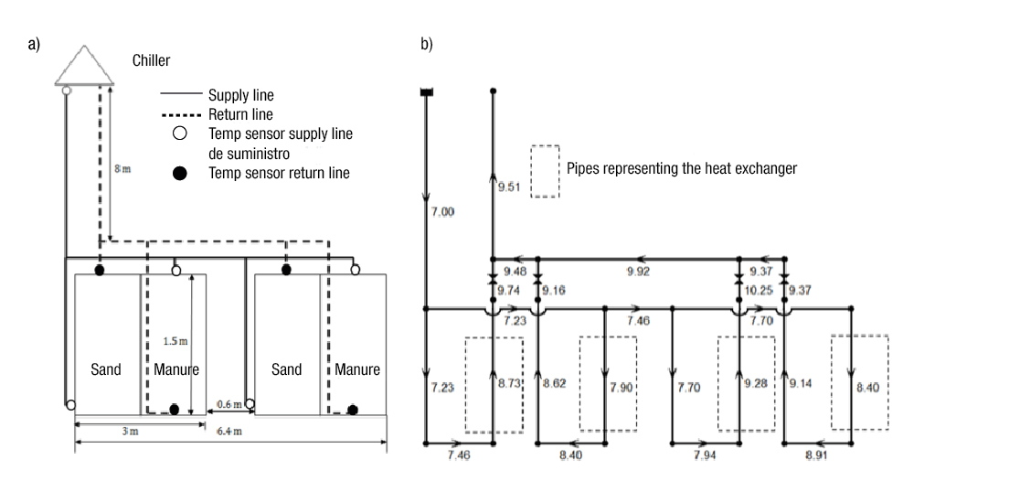
Figure 3 a) Scheme of the experimental pipe network used to test the conductive cooling system; b) Water temperature predictions achieved by the heat transfer solver implemented in EPANET as water moves along the pipes using hot-and-humid ambient conditions and dried manure for bedding.
Temperature data loggers (HOBO U12, Onset Computer Corporation, USA) were placed at the supply and return water lines for each individual bed. These data loggers were set to record measurements with a 15 min time step. Four Holstein dairy cows were used in the experiment for a period of 80 days. The experiment was divided into two periods of 40 days each, and each period consisted of three repetitions of three different climate scenarios (Hot Dry, Thermo-neutral and Hot Humid). At the beginning of each period, the cows were allowed an acclimation phase of seven days. Each repetition consisted of nine days (three days per climate), and after each repetition, the cows were allowed three days to reset their thermo-neutral conditions; further information is found in Xavier et al. (2015).
Results and discussion
Validation of the heat transfer solver
Datasets related to ambient, bedding and water temperatures were filtered discarding measurements having changes larger than ± 0.4 °C in a period of 15min. With these settings in place, the conductive cooling system was tested with respect to three different ambient conditions: thermo-neutral, hot and dry, and hot and humid. For each case, the average temperature of the pipe network obtained in the experiment was calculated, as well as the simulated data (Table 1). Such data were obtained under steady-state conditions reached during a 24-h period; additional information about the experiments is provided in Ortiz et al. (2015). Simulation results were in good agreement with experimental data (≤ 0.6 °C), thus proving that the heat transfer solver can reliably predict the temperature of water circulating through a conductive cooling system in operation in a dairy barn.
Table 1 Average water temperature recorded during 24 h under different ambient conditions and bedding materials.
| Ambient conditions | Mean ambient temperature | Bed temperature | Experimental water temperature | Simulated water temperature | |||
|---|---|---|---|---|---|---|---|
| (°C) | |||||||
| - | Dried manure | Sand | Dried manure | Sand | Dried manure | Sand | |
| Thermo-neutral | 20.0 | 20.5 | 18.1 | 8.8 | 9.7 | 8.8 | 9.8 |
| Hot and dry | 40.0 | 31.2 | 29.0 | 9.5 | 10.8 | 9.0 | 10.4 |
| Hot and humid | 30.0 | 30.5 | 28.4 | 9.4 | 10.9 | 9.6 | 10.7 |
As a particular case, experimental and simulated data were compared for the hot-and-humid scenario and using dried manure as bedding. Figure 3 presented the temperature prediction as water moves through each pipe segment using the heat transfer module.
Simulation of a large-scale pipe network
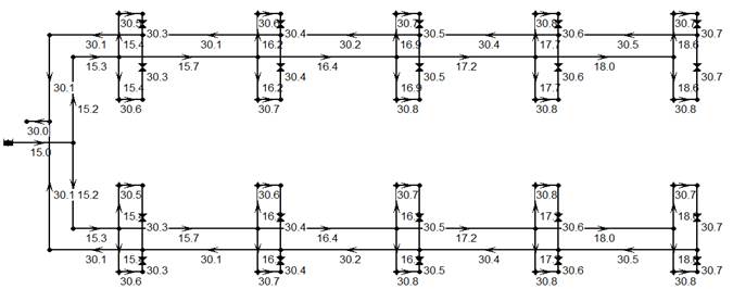
The following example is related to a proposal for a large-scale system that may potentially operate in an average dairy barn equipped with 1 000 HEs uniformly distributed across a floor area of 8 600 m2. To make it realistic, the present design follows dimensions and components in accordance with the American Society of Agricultural and Biological Engineers (ASABE, 2010). Specifically, this design has two parts: 1) 20 clusters, each containing 50 HEs (Figure 4), and 2) the main line (Figure 5), which provided water to each of the 20 clusters. Each cluster was located on a surface of 38 m in length and 5.3 m in width and was arranged in two lines of 25 HEs, the rows 1.5 m apart and the HEs spaced 2.5 m apart.
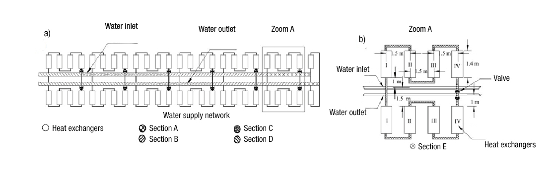
Figure 4 Pipe network: a) a cluster of 50 heat exchangers and b) zoom of zone A, detailed description of a cluster of eight HEs connected to the inlet and outlet of the cluster main lines.
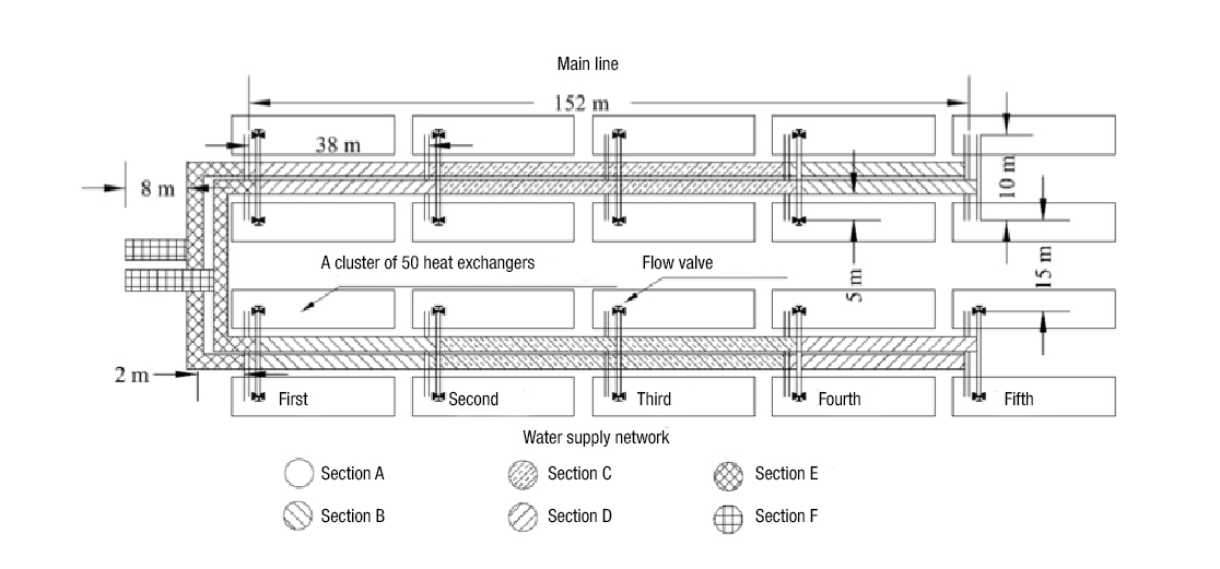
The HEs in each cluster were first connected in parallel and then in a serial configuration; a repeated grouping of eight interconnected HEs (Figure 4), where a set of four HEs were connected in series on one side and another set of four were placed in parallel on the opposite side. To set the required flow rate, a flow-control valve was placed at the end of each set. The path delivering water was thus similar to the path returning it to the point of origin. Since this system was used for cooling purposes, water running through the fourth HE had to cool a cow with heat fluxes between 150 and 700 W·m-2.
Specifications related to clusters and main pipe line are listed in Table 2; the diameters corresponded to velocities between 0.05 and 2 m·s-1, which covered flow rates demanded in each HE (between 1 and 7 L·min-1). The pipe wall thermal conductivity equaled 0.19 W·m-1·°C-1. A pipe wall roughness of 0.5 x 10⁻⁵ m was assumed, and the Darcy-Weisbach equation was used to compute local heat losses (US EPA, 2008). Energy losses occurring in each pipe and minor local losses occurring at junctions were included in order to find the total amount of energy required to pump water through the whole loop. Feasible operational range will involve a range of pumping rates.
Table 2 Pipe specifications.
| Pipe | Diameter | Pipe wall thickness |
|---|---|---|
| (mm) | ||
| Section A | 15.8 | 2.8 |
| Section B | 21.0 | 2.9 |
| Section C | 27.0 | 3.4 |
| Section D | 35.0 | 3.6 |
| Section A | 52.1 | 3.9 |
| Section B | 78.0 | 5.5 |
| Section C | 102.3 | 6.0 |
| Section D | 154.0 | 7.1 |
| Section E | 254.5 | 9.3 |
| Section F | 303.2 | 10.3 |
Pipes in the setup shown in Figures 4 and 5 were assumed to have a constant external pipe wall temperature of 26.7 °C (corresponding to the case of the maximum monthly temperature for soil at a depth of 0.5 m for Tucson ENT#091;AZMet, 2012ENT#093;). The initial water temperature was set at 15 °C as the typical water temperature observed in wells in Tucson. Then, a section of the pipe network transported water at a temperature that was lower than the external pipe wall temperature, thus causing a heat gain. Once water temperature became higher than the external pipe wall temperature, the heat exchange reversed.
For this pipe network, all HEs were governed by Equations 1 to 10. It was also assumed that all HEs were rectangular ducts of a length equal to 1.4 m, a width equal to 0.8 m, and a height equal to 0.051 m. For proper representation of a HE, some parameters were changed: dy (0.02 m), K p (2 W·m-1·°C-1), S (1.12 m2), and P (0.096 m). In Equation 7, since flow in each HE was within the laminar flow regime in rectangular ducts, the equation coefficient of 3.66 was changed to 4.86. It was assumed that surface S would be able to maintain a constant temperature T i,epw equal to 35 °C. Data related to thickness and thermal conductivity of the HE and bedding material were comprised in the values for dy and K p . Pressure drops occurring at the HE did not differ significantly from that of a pipe with a diameter of 0.227 m; to prove this fact, Mondaca et al. (2013) simulated water flowing within a HE by means of fluid dynamics.
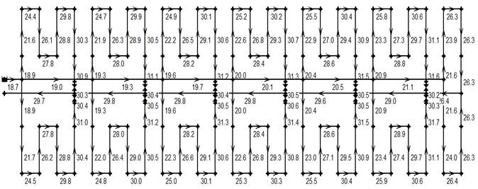
Heat transfer rates computed should help to illustrate the temperature variations that occurred over the entire system (Figure 6), and also variations that occurred among clusters located in the fifth column (Figure 7). Note that, as consequence of the pipe network design, the EPANET hydraulic module generated key parameters such as water velocity, flow rates, and pressure drop in each pipe segment. The critical cluster at the end of the main line registered the highest temperature (18.6 °C) after passing water through the HE; however, cooling was still above the critical minimum cooling capacity of 150 W·m-2 reported by Mondaca (2013).
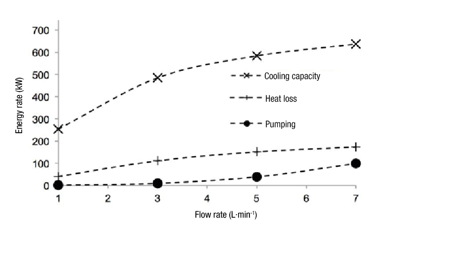
Given that water temperature changed as water passed through the pipe network, cooling capacity in each HE may vary according to its location within the cluster. The locations at which the lowest and highest water temperatures occurred imply the maximal and minimal cooling capacity possible, given the effects of the water flow rates supplied to the HE. We assumed that the entire set of HEs would receive the same flow rate but water temperature would vary because each HE was at a different location in the pipe network. Thus, the flow rate not only affected cooling capacity but also the amount of energy required for pumping (Figure 8). Pumping needs can be found by using the equation taken from Mays (2000) with efficiency of the pump set equal to 100 %. Cooling capacity refers to the performance of the HEs, and total heat lost can be computed by measuring heat transfer that occurs during water transportation.
The energy rate required to pump the water, heat losses by transportation and cooling capacity can determine overall efficiency, which can be found by Equation 11.
Average amount of heat lost in any cluster and also throughout the entire system depends on the thickness of the material for insulating pipes and HEs installed for conductive cooling. Distance between clusters and HEs as well as the amount of insulation can determine how efficient the system will be. The present example considers no insulation in pipes and then two levels of insulation by reducing thermal conductivity in pipes to show that the system’s performance can be enhanced. Figure 9 indicates that during periods of low flow rate (1 and 7 L·min-1), the system’s efficiency could have improved even though low flow rates decrease the cooling capacity significantly.
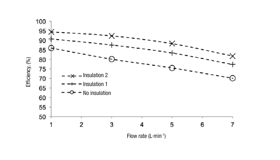
Figure 9 Insulation to reduce heat loss: ‘No insulation’ corresponds to pipe wall thermal conductivity, ‘Insulation 1’ and ‘Insulation 2’ correspond to reductions of 50 and 75 %, respectively, in the thermal conductivity at the pipe wall.
Additionally, it was found that thermal conductivity for Insulations 1 and 2 with values of 0.095 and 0.0475 W·m-1·°C-1, respectively, increased by 7 and 12 %, respectively, for a flow rate of 7 L·min-1. In contrast, if flow rate was 1 L·min-1, efficiency increased by 5 and 8.4 % for Insulations 1 and 2, respectively. These results showed that insulation can enhance the system’s efficiency, and it should be considered when external pipe wall temperature or pipe lengths are affecting thermal performance.
These findings can be seen as promising in terms of the feasibility of building a large-scale conductive cooling system, even though it was demonstrated only for four HEs in controlled conditions in Ortiz et al. (2015). However, it is suggested that additional issues may arise related to decrease of insulation effectiveness due to moisture around the pipe network, cow’s habits to lie down, maintenance required and cost of operation. That kind of information can be obtained in further investigations when installing such system in real dairy barn conditions.
Conclusions
A pipe network layout that can satisfy hydraulic requirements was the basis for determining the thermal energy needed to efficiently operate a conductive cooling system. A well-designed pipe network can accurately simulate transportation of water and heat transfer. Combined hydraulic and thermo-physical parameters enabled the pipe network to predict water temperature.
The model was partially validated since experiments were conducted for a group of four HEs in order to confirm validity of heat transfer. Large-scale experimental tests were not conducted; however, it must follow the same principles of heat transfer. Thus, predictions of water temperature in a large-scale pipe network to cool down 1 000 cows using conductive cooling beds can be suggested to determine the system’s pumping needs, heat transfer performance, and also the system’s overall efficiency.
According to the findings of this investigation, a low flow rate will reduce cooling capacity but increase efficiency; therefore, any similar design should be operated at a flow rate that enables HEs to achieve sufficient cooling while maximizing energy savings. This criterion applies to cases where time response is not a constraint. Since efficiency diminishes when the water must travel long distances, even if the system is adequately insulated, a system’s size should depend on how much heat can be lost without unduly impairing the system’s operation.
In general, the conductive cooling system is viable in areas with a desert climate and its efficiency depends on the level of thermal insulation and flow in the pipe network. Further research could help to more precisely determine the consequences associated with system size and to what extent insulation can help to reduce heat losses and guarantee that water will be supplied to the HEs at the desired temperature.

