


 text in
  English (pdf)
 Article in xml format
 Article references
 Send this article by e-mail
 Cited by SciELO
  Similars in
SciELO
Similars in
SciELO 
 Permalink
Introduction
The global area under irrigation is about 20 %, mainly located in arid and semi-arid areas that show high spatial and temporal variability conditions in the available volumes of their sources of supply and that thus require irrigation to ensure commercial returns (Food and Agriculture Organization [FAO], 2011). In Mexico, irrigated agriculture is concentrated in coastal areas that are highly vulnerable to the effects of climate variability and change, particularly extreme weather events such as hurricanes, frost, drought, etc. (Ojeda-Bustamante, Sifuentes-Ibarra, Iñiguez-Covarrubias, & Montero-Martínez, 2011).
Corn is the basic input of the Mexican diet. Approximately 60 % of corn production is intended for human consumption, with a per-capita value of 127 kg·year-1 (Nadal & Wise, 2005), and the area annually cultivated is 7 to 8.5 million hectares, where 85 % of this area is under rain-fed conditions and 15 % under irrigation (Muñoz-Pérez & Hernández-Rivera, 2004). However, irrigated corn is 3.5 times more productive than rain-fed corn.
In Mexico, the state of Sinaloa is the leading producer of irrigated corn, sowing 400 to 500 thousand hectares annually in its eight irrigation districts, with production of 3.5 to 5 million tons (Comisión Nacional del Agua [CONAGUA], 2015); however, although Mexico is one of the world’s leading corn producers, its consumption of this grain is higher than its production thereof, so it is one of the major importing countries, requiring more than 7 million tons per year (Servicio de Información Agroalimentaria y Pesquera [SIAP], 2016).
In Mexico, the application of water at plot level is poor when mainly surface irrigation is used, usually in the form of furrows, without design, layout and monitoring in accordance with technological advances, so there is pressure to optimize plot irrigation (Ojeda-Bustamante, Sifuentes-Ibarra, Rojano-Aguilar, & Íñiguez-Covarrubias, 2012). It is estimated that less than 45 % of the water applied to the plots is productively used; the rest is lost by drainage and deep percolation, with the consequent loss of mobile fertilizers and soil (Ojeda-Bustamante et al., 2012). Restrictions on water use for irrigation are common due to recurrent periods of low availability, subjecting crops to water stress.
In corn, water deficiencies cause detrimental effects on yield in relation to their intensity and the crop’s phenological stage (Claassen & Shaw, 1970). Cakir (2004) evaluated the effects of water stress on the vegetative stage of corn for three years, obtaining biomass reductions of 28 to 32 %, but reported no significant differences in yield of the treatments compared to the control (without water deficit).
In corn, the flowering and grain filling stages are considered critical to ensure optimum yields (Pasquale, Hsiao, Fereres, & Raes, 2012). Because of this, the presence of high temperatures, combined with periods of water stress, can affect the processes of pollination, fertilization and grain development (Bassetti & Westgate, 1993; Wilhelm, Mullen, Keeling, & Singletary, 1999; Suzuki, Tsukaguchi, Takeda, & Egawa, 2001). The phenological stage most sensitive to water stress is male flowering (Cakir, 2004), and it can reduce biomass production by 30 % and grain yield by 40 %.
During reproductive development, water stress reduces the number of grains due to a decrease in the rate of photosynthesis and the flow of assimilates to the developing organs of the crop (Schussler & Westgate, 1995). Flowering and the initial stages of grain filling in corn are considered critical in determining grain yield.
Pasquale et al. (2012) updated the Doorenbos and Kassam (1979) guide from experimental data published in various parts of the world on the response of crops to irrigation applied, based on their phenological stage. However, evaluation of the impact of water stress on crops must be done locally for its transfer and adoption to ensure production in an irrigated area.
Deficit irrigation is a technique studied and used in various regions of the world with water availability problems (Chai et al., 2016). This involves a reduction in irrigation, below potential crop water demands, which is applied during phenological stages with greater tolerance to water stress (Ojeda-Bustamante et al., 2012). This technique has shown advantages for its water-saving potential (Rázuri, Romero, Romero, Hernández, & Rosales, 2008; Chai et al., 2014).
Hargreaves and Samani (1984) indicated that deficit irrigation can provide better economic returns per unit area, equal to or greater than those obtained under full irrigation for maximum yield, which clearly creates greater efficiency in water use. Although this type of irrigation has been successfully applied in various parts of the world, its adoption requires local validation. In the case of Mexico, there is limited information on the response of different crops to deficit irrigation, although there have been reports on paprika, chili and peach by Rodríguez-Padrón, Rázuri-Ramírez, Sworowsky, and Rosales-Daboín (2014), Serna-Pérez and Zegbe (2012) and Tapia-Vargas et al. (2010), respectively.
Given the recurrent droughts and their intensification with climate change, which will impact the availability of water for irrigation, it is necessary to study the potential for applying deficit irrigation to generate water savings under current and future conditions in Mexico for crops of national importance (Ojeda-Bustamante et al., 2011).
It is possible to reduce irrigation depths if the crop is subjected to regulated water stress in phenological stages with tolerance to this, without substantially affecting potential yield. Therefore, the aim of this research was to evaluate the deficit irrigation technique in corn under furrow irrigation in an irrigation area of Mexico for practical application to help increase efficiency in water use. Three water deficit levels were used: 10, 20 and 30 %, labeled as T1, T2, T3, respectively, and the control treatment (C), wherein the irrigation requirement demanded by the crop was applied.
Materials and methods
The work was carried out during the 2012-2013 autumn-winter (O-W) crop cycle, at the Valle del Fuerte Experimental Station (CEVAF) operated by the National Institute for Forestry, Agricultural and Livestock Research (INIFAP) in the arid zone of northern Sinaloa, Mexico, with geographical coordinates of 25° 48’ 39.6’’ north latitude, 109° 01’ 30’’ west longitude and at 20 masl. The experiment was carried out in soil typical of the region: clayey texture, usable volumetric moisture of 0.155 cm-3, bulk density of 1.15 g·cm-3 and organic matter content of 1 %. The plot is part of irrigation district 075, Rio Fuerte, Sinaloa, one of the largest irrigation districts in Mexico (CONAGUA, 2015). Annual cumulative rainfall in the study area is 350 mm, which is concentrated from July to September with 70 % of the cumulative rainfall in the year, while the amount that falls from February to May is negligible. The annual values of cumulative reference evapotranspiration (ETo) range from 1600 to 1700 mm; this exceeds the precipitation throughout the year and, therefore, irrigation is required to ensure commercial returns.
The cumulative precipitation during the intermediate corn crop cycle, lasting 191 days after sowing (das), was 42.4 mm, with 37.8 mm concentrated in the month of December, which corresponds to the planting month, and was taken into account when estimating irrigation requirements. The average maximum, median and minimum temperatures in the cycle were 29.61, 20.30 and 11.83 ºC, respectively. The ETo was 947.7 mm with 1,898 cumulative degree days (ºDA). These meteorological data were obtained from the automated weather station installed 100 meters from the site of the experiment.
For real-time irrigation scheduling, the IrriModel computer system, an improved version of the Spriter computer tool (Ojeda-Bustamante, González-Camacho, Sifuentes-Ibarra, & Rendón-Pimentel, 2007), was used. This software offers the following benefits: 1) calculates crop water demand, 2) generates irrigation schemes under different water availability scenarios and types of irrigation systems, 3) predicts irrigation using a water balance model with a high level of accuracy, according to the phenological development of the crop, using the concept of degree days (ºD), documented by Ojeda-Bustamante, Sifuentes-Ibarra, and Unland-Weiss (2006), and 4) facilitates tracking the irrigation on one or more plots in an agricultural cycle.
The total area of the experimental plot was 1.72 ha, in which four treatments (Tn) with five replications were established. The treatments consisted of reducing the applied irrigation depth, recommended by the IrriModel software, to generate deficit in the phenological stages less sensitive to water stress using surface irrigation (furrows). Each treatment had the same water deficit throughout its phenological stages except the flowering stage (R1), in which the treatments received normal irrigation. The water deficit levels applied were, respectively, 10, 20, 30 and 0 %, for T1, T2, T3 and C (Table 1). Monitoring of crop phenological stages was carried out in accordance with the work of Abendroth et al. (2009) and Ojeda-Bustamante et al. (2006).
Table 1 Application of irrigations in phenological stage in which the treatments were subjected to water stress.
| Irrigation | Phenological stage | Water deficit treatments (%) | |||
|---|---|---|---|---|---|
| T1 | T2 | T3 | C | ||
| 1 | V6 | 10 | 20 | 30 | 0 |
| 2 | R1 | 0 | 0 | 0 | 0 |
| 3 | R2 | 10 | 20 | 30 | 0 |
| 4 | R3 | 10 | 20 | 30 | 0 |
V6= six true leaves, R1 = flowering, R2 = aqueous grain, R3 = milky grain
Water deficit levels used in this study were similar to those used by Rázuri et al. (2008) in four treatments, which consisted of supplying different water volumes (depths), which corresponded to the recovery of 100, 80, 70 and 60 % of crop evapotranspiration (ETc) in tomato under localized irrigation, and they reported that there were no significant differences in yields between treatments, although the 80 % one presented better commercial fruit quality.
Optimal furrow length and flow were estimated with the RIGRAV 3.0 program developed by Rendón, Fuentes, and Magaña (1997), according to the conditions and variables of the experimental site. The main method of applying irrigation in the area is by furrows through siphon-shaped pipes at the head end of each furrow. The flow was applied in the furrows with siphons, for which the load to obtain the required flow was set, according to the load-flow curve of the previously calibrated siphons. In general, producers do not have rigorous control over the load input to the furrows, resulting in great variation in the flows and volumes applied to each one.
The corn crop was planted on a dry basis on December 12, 2012 using a precision seeder, and the next day germination irrigation was applied. The intermediate-cycle DK-3000 variety was planted. In T1, T2 and T3, prior to planting, fertilizer based on 250 kg·ha-1 of physical mixture of 30-10-12 of N-P-K, respectively, was applied, while 450 kg·ha-1 of the same product was supplied to C, in accordance with the practices of the leading producers in the area. During the appearance of the fifth true leaf (V5), supplementary fertilization consisting of 100 kg·ha-1 urea (46-00-00) was applied in all treatments, including the control. The seeding density was 100,000 seeds·ha-1, with plants spaced 12.5 cm apart. When the crop reached 50 cm in height, we proceeded to plant and open furrows simultaneously to apply auxiliary irrigations based on the water deficit treatments.
For the initial irrigation the volumetric moisture of the soil was estimated with a calibrated Time Domain Reflectometry (TDR) sensor, after which the irrigation depth required to bring the soil to field capacity (FC) was calculated. For the rest of the auxiliary irrigations, IrriModel software was used to estimate the date and net irrigation depths (L n ), according to the deficit treatments, using the methodology presented by Ojeda-Bustamante et al. (2006).
The irrigations were assessed in terms of application efficiencies (E a , %), using the formula E a = (L n / L b ) X 100, where L n is the net depth required and L b the gross or applied depth (m) (Bolaños-González, Palacios-Vélez, Scott, & Exebio-García, 2001). The estimation of L b was calculated using the equation L b = (Q T) / A, where Q is the irrigation flow applied to the plot (m3·s-1), T is the irrigation time (s) and A is the irrigated area (m2) (Martin, 2001).
Water productivity (WP) and yield (Y) of the treatments were also estimated. The former indicates the ratio of the total production obtained (RC, kg) with respect to the total volume of water applied (AV, m3) (Bessembinder, Leffelaar, Dhindwal, & Ponsioen, 2005) and the latter the production obtained in kg·ha-1.
Harvesting took place on June 20, 2013, corresponding to 191 das or 1,898 ºDA, from sowing to harvest, in accordance with the work of Ojeda-Bustamante et al. (2006). Five samplings were performed to estimate yield in representative sites located in the two central furrows of each treatment in a7.6 m2 area, per site. This procedure was performed in all treatments, including the control.
To determine the significant difference in the yields, analysis of variance for comparison of means was performed with the Tukey test (P ≤ 0.05), using a randomized block design and the Statistical Analysis System statistical package version 9.2 (SAS, 1999).
The relative difference Δ in the four response variables of interest of the treatments (ΔY, ΔL b , ΔEa and ΔWP), with respect to the control, corresponding, respectively, to Y in t·ha-1, Lb in cm, Ea in percentage and WP in kg·m-3, was calculated using the following general relationship:
where T n is the treatment n, C is the value obtained from the control.
As an example, for the case of the relative difference in yield, the equation for ΔY would be:
where Y n is the yield of treatment n and Y C is the yield obtained in the control.
Results and discussion
In each treatment a total of five irrigations was applied. The initial depths were 10.9, 10.0, 10.0 and 14.7 cm, for T1, T2, T3 and C, respectively.
Irrigations applied to T1 (10% water deficit) throughout the crop cycle are presented in Table 2. It can be seen that the auxiliary irrigations, in terms of L n , fluctuated between 11.3 and 14.8 cm L b , applying a cumulative depth of 63 cm, representing 2,792 m3 with 63 % Ea, throughout the crop cycle. Reducing irrigation depth applied by deficit irrigation improves the efficiency of water use in corn throughout the crop cycle. Reducing the irrigation depth applied by deficit irrigation improves the efficiency of water use in corn, as reported by Chai et al. (2016).
Table 2 Irrigation scheduling applied for T1
| NI | Start | Time (h) | Flow (L·s-1) | Area (ha) | Volume (m3) | L n (cm) | L b (cm) | Ea (%) |
|---|---|---|---|---|---|---|---|---|
| 1 | 12/12/2012 | 3.2 | 42 | 0.4332 | 553 | 5.5 | 10.9 | 50 |
| 2 | 01/03/2013 | 2.3 | 59 | 0.4332 | 487 | 6.75 | 11.25 | 60 |
| 3 | 24/03/2013 | 3.0 | 34 | 0.4332 | 498 | 8.1 | 11.50 | 70 |
| 4 | 09/04/2013 | 4.5 | 25 | 0.4332 | 615 | 9.95 | 14.20 | 70 |
| 5 | 27/04/2013 | 2.5 | 43 | 0.4332 | 639 | 9.72 | 14.75 | 66 |
| Total | 2,792 | 40 | 63 | 63 | ||||
NI: number of irrigations, L n : net depth, L b : gross depth, Ea: application efficiency
Irrigations applied to T2 (20 % water deficit) are presented in Table 3. It can be seen that the auxiliary irrigations fluctuated between 10.5 and 13.5 cm L b , applying 57 cm of cumulative depth, representing 2,460 m3 of total volume with 65 % Ea. It is also observed that from the second auxiliary irrigation the application efficiency increases. The depth applied in this treatment coincides with the results obtained by (Rivetti, 2006), with a gross consumption of 57 cm throughout the corn crop cycle.
Table 3 Irrigation scheduling applied for T2
| NI | Start | Time (h) | Flow (L·s-1) | Area (ha) | Volume (m3) | L n (cm) | L b (cm) | Ea (%) |
|---|---|---|---|---|---|---|---|---|
| 1 | 13/12/2012 | 3.2 | 43 | 0.43 | 430 | 5.5 | 10.0 | 55 |
| 2 | 28/02/2013 | 2.5 | 59 | 0.43 | 452 | 6.0 | 10.5 | 57 |
| 3 | 24/03/2013 | 2.6 | 38 | 0.43 | 439 | 7.2 | 10.2 | 71 |
| 4 | 09/04/2013 | 4.6 | 29 | 0.43 | 558 | 10.0 | 13.0 | 77 |
| 5 | 27/04/2013 | 2.5 | 58 | 0.43 | 581 | 8.6 | 13.5 | 64 |
| Total | 2,460 | 37.3 | 57 | 65 | ||||
Ni: number of irrigations, L n : net depth, L b : gross depth, Ea: application efficiency
Irrigations applied to T3 (30 % water deficit) are presented in Table 4. The auxiliary irrigations fluctuated between 8.5 and 11.5 cm L b , applying 50 cm of cumulative gross depth, representing 2,150 m3 of total volume with 69 % Ea. Reducing irrigation depth increases plot efficiency and possibly the use of nutrients available in the soil, thereby increasing grain yield as reported by Hargreaves and Samani (1984).
Table 4 Irrigation scheduling applied for T3
| NI | Start | Time (h) | Flow (L·s-1) | Area (ha) | Volume (m3) | L n (cm) | L b (cm) | Ea (%) |
|---|---|---|---|---|---|---|---|---|
| 1 | 13/12/2012 | 3.2 | 43 | 0.43 | 430 | 5.5 | 10.0 | 55 |
| 2 | 28/02/2013 | 2.3 | 40 | 0.43 | 366 | 5.3 | 8.5 | 62 |
| 3 | 24/03/2013 | 2.3 | 40 | 0.43 | 387 | 7.2 | 9.0 | 80 |
| 4 | 09/04/2013 | 4.7 | 30 | 0.43 | 495 | 9.7 | 11.5 | 85 |
| 5 | 27/04/2013 | 3.0 | 60 | 0.43 | 473 | 6.9 | 11.0 | 62 |
| Total | 2,150 | 34.6 | 50 | 69 | ||||
NI: number of irrigations, L n : net depth, L b : gross depth, Ea: application efficiency
Gross irrigations applied to C fluctuated between 14.3 and 15.6 cm L b , applying 73.5 cm of cumulative gross depth, representing 3,159 m3 of total volume with 58 % Ea (Table 5). The irrigations and depths supplied in this treatment were based on conventional application and management techniques followed by the agricultural leaders in the study area. These data are similar to those reported by Ojeda-Bustamante et al. (2006) in corn, where the greatest losses occurred due to runoff and percolation.
Table 5 Irrigation scheduling applied for C
| NI | Start | Time (h) | Flow (L·s-1) | Area (ha) | Volume (m3) | L n (cm) | L b (cm) | Ea (%) |
|---|---|---|---|---|---|---|---|---|
| 1 | 12/12/2012 | 8.0 | 22 | 0.43 | 631 | 5.5 | 14.7 | 37 |
| 2 | 28/02/2013 | 7.9 | 26 | 0.43 | 671 | 7.8 | 15.6 | 50 |
| 3 | 24/03/2013 | 4.5 | 29 | 0.43 | 559 | 9.0 | 14.5 | 69 |
| 4 | 09/04/2013 | 6.9 | 23 | 0.43 | 602 | 9.8 | 14.4 | 70 |
| 5 | 27/04/2013 | 5.0 | 29 | 0.43 | 602 | 10.8 | 14.3 | 77 |
| Total | 3,159 | 42.9 | 73.5 | 58 | ||||
NI: number of irrigations, L n : net depth, L b : gross depth, Ea: application efficiency
Figure 1 compares the average yields obtained in each treatment, which were: 11.04, 11.05 and 11.44 t·ha-1, for T1, T2 and T3, respectively. For C the yield was 11.87 t·ha-1. No significant difference between treatments with respect to C was found, despite the fact that in C an additional 200 kg·ha-1 of fertilizer was applied, in accordance with local practice. The results of this research work are similar to those reported by Farré (2010) in corn under deficit irrigation.
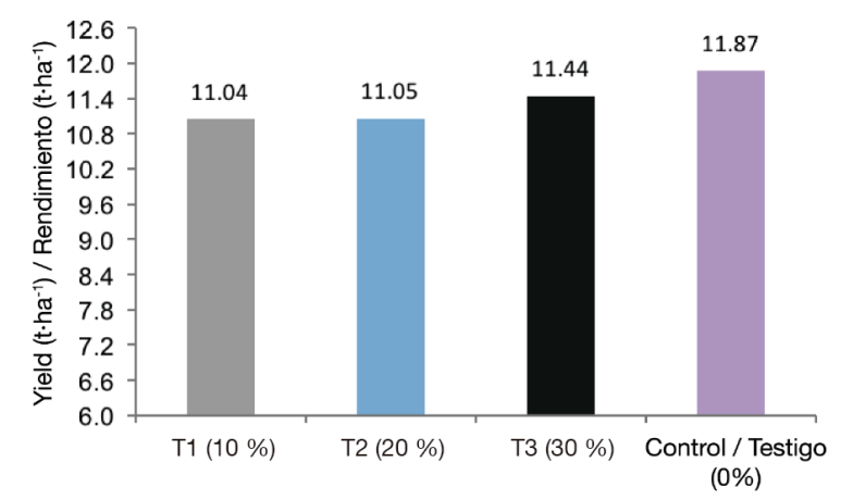
Figure 2 shows the water productivity obtained for each treatment. T3 had the highest productivity with 2.29 kg·m3 of grain, compared with C that had the lowest value with 1.61 kg·m3. This indicates that the water deficit technique is viable if reduced or avoided at critical crop stages such as flowering. These results are similar to those reported by Rivetti (2006) in corn in deficit irrigation research.
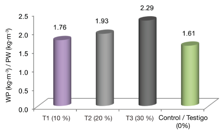
Table 6 shows the statistical comparison of yields and, as can be seen, there was no significant difference in yield in the five replications of the three treatments and the control.
Table 6 Results of comparison of means obtained per treatment for five replications
| Treatments | R1 | R2 | R3 | R4 | R5 |
|---|---|---|---|---|---|
| T1 (10 %) | 10.56 a | 10.79 a | 10.62 a | 11.82 a | 11.38 a |
| T2 (20 %) | 10.07 a | 12.2 a | 10.23 a | 11.17 a | 11.58 a |
| T3 (30 %) | 11.47 a | 10.92 a | 11.07 a | 11.88 a | 11.86 a |
| TES (0 %) | 11.59 a | 11.91 a | 11.95 a | 11.56 a | 12.36 a |
Note: Means indicated with the same letter in a column are not significantly different according to the Tukey test (P ≤ 0.05), with a coefficient of variation of 4.5.
Table 7 shows the relative differences in the variables ΔY, ΔL b , ΔEa and ΔWP. It is observed that increasing the water deficit levels increases the ΔEa and ΔWP, and reduces the ΔL b , without drastically affecting yields. The results indicate that regulated deficit irrigation is a viable way to improve efficiency and productivity through better use of water, as has been similarly reported by Chai et al. (2016).
Conclusion
For the full-irrigation control, although an additional 200 kg of nitrogen fertilizer were applied to it, no significant differences in yield with respect to the water deficit treatments were found. It turned out that the treatment with the greatest water deficit, T3 (30% water deficit), was the best treatment, from the point of view of efficiency, savings, water productivity and yield. This indicates that regulated deficit irrigation in corn under furrow irrigation is an alternative that helps increase efficiency in water use in agriculture. It is also an option to deal with the scenario of water scarcity in the irrigation area studied.
Deficit irrigation is an easy technique to apply and manage when there is enough field information to generate robust irrigation scheduling. However, one cannot generalize the use of treatments for different types of soils; it is therefore recommended to locally validate its application for each irrigation area and specific crop

