


 text in
  English (pdf)
 Article in xml format
 Article references
 Send this article by e-mail
 Cited by SciELO
  Similars in
SciELO
Similars in
SciELO 
 Permalink
Introduction
Several tools and techniques have been developed for measuring climatic elements in order to know the current weather (Gutiérrez, García, Magaña, & Escalante, 2007) and provide information for short-term forecasting, statistical analysis, farm support, air and maritime navigation safety, and characterization and classification of the weather and atmospheric state at a particular time and place. A meteorological instrument is the combination of a sensitive element and a system able to convert measurements of this element into a numerical value, which represents the meteorological variable being evaluated. The representative area of a region having meteorological equipment, at which climatic elements can be observed, measured, recorded, concentrated and processed, is commonly referred to as a weather station (Nájera & Arteaga, 1998).
Often weather station records for a certain period are incomplete due to the absence or replacement of the operator, recording device failures or operational negligence (Aparicio, 2007; Campos-Aranda, 1998), which has limited the conducting of agro-climatic studies whose results enable increasing productivity, optimizing resources, reducing the risk of crop loss, planning irrigation and drainage infrastructure in an integrated manner and making weather forecasts (Toro-Trujillo, Arteaga-Ramírez, Vázquez-Peña, & Ibáñez- Castillo, 2015). According to the World Meteorological Organization (OMM, 2011), the planning and implementation of user projects cannot be deferred until there are sufficient meteorological or climatological observations; therefore, estimation is used to expand, fill in or complete the information. It also recommends that the study period be at least 30 years.
Among the most common methods for estimating missing data series are: normal ratio (NR), which is used when the mean annual precipitation of any of the neighboring stations differs by more than 10 % (Aparicio, 2007), and when it differs by less than 10 % it is estimated with the arithmetic average of the records of the neighboring stations (Alfaro & Pacheco, 2000; McCuen, 1998). Aparicio (2007) recommends using at least three auxiliary stations in both cases.
The WMO (2011), Campos-Aranda (2015), Allen, Pereira, Raes, and Smith (2006) and DeGaetano, Eggleston, and Knapp (1995) propose using linear regression (LR) and multiple regression (MR). The latter consists of obtaining a mathematical equation that expresses the relationship between the dependent variable (Y) and the independent one (X), or explanatory variables (X1, X2... Xn), although rarely is a perfect linear relationship observed because the phenomena studied in climatology are usually nonlinear, so both records must be homogeneous; that is, they need to represent the same conditions. When there are no stations surrounding the station with missing information, the missing values are deduced with the deductive rational (DR) method proposed by Campos-Aranda (1998), which allows estimating them with the information provided by the complete years of the same series (Puertas- Orozco, Carvajal-Escobar, & Quintero-Angel, 2011).
The method most used in hydrological and geographical studies is the U.S. National Weather Service’s inverse square distance (ISD) method (Ramírez-Cruz, López- Velasco, & Ibáñez-Castillo, 2015). In this case, the influence of rain at a station for the calculation thereof at any point is inversely proportional to the distance between the station and the auxiliary stations (OMM, 2011). The most significant advantage of the ISD method is that it uses daily data, grouped into periods of five or ten days, monthly or yearly (Teegavarapu & Chandramouli, 2005; Toro-Trujillo et al., 2015).
Other procedures include moving averages (Campos- Aranda, 1998) and autoregressive, logarithmic, and triangulation methods, all based on normality assumptions. According to the WMO (2011), there are also estimation methods known as geostatistics based on theoretical foundations, which are statistical assumptions. The most important are the Kriging and optimal interpolation methods. The former is a spatial interpolation method based on showing the proportion at which the variance changes between points in space, and is expressed in a variogram. These procedures are limited by requiring a certain amount of data to produce a reliable and appropriate variogram (Toro-Trujillo et al., 2015). In addition, Wagner, Fiener, Wilken, Kumar, and Schneider (2012) suggest that these procedures do not represent an improvement over the ISD method.
To evaluate and select the method that best fits the variable analyzed, there are various tests and procedures known as statistical indices, which consist of estimating the error or bias; some of them are: the mean standard error or root mean square error (RMSE), the Willmott index of agreement (d) (Willmott, 1981), the coefficient of determination (R2) and the relative error (RE) (Cervantes-Osornio, Arteaga-Ramírez, Vázquez- Peña, Ojeda-Bustamante, & Quevedo-Nolasco, 2013; Kelso-Bucio, Bâ, Sánchez-Morales, & Reyes-López, 2012; Wright, 2001; Cai, Liu, Lei, & Pereira, 2007).
The aim of this study was to compare the deductive rational (DR), normal ratio (NR) and United States Weather Services’ inverse square distance (ISD) methods, and then select the best one to estimate the missing daily precipitation and maximum and minimum temperature data at weather stations located in San Luis Potosí, Mexico.
Materials and methods
Description of the study area
The state of San Luis Potosí is located in the Central Mexican Plateau. Its extreme geographical coordinates are: 24° 29’ and 21° 10’ north latitude, 98° 20’ and 102° 18’ west longitude. This area accounts for 3.2 % of the country’s total area (Instituto Nacional para el Federalismo y Desarrollo Municipal [INAFED], 2010), and because of its climatic and morphological diversity, the state is divided into four geographical regions: Altiplano, Centro, Media and Huasteca (Instituto Nacional de Estadística y Geografía [INEGI], 2007).
Climatological databases
The databases used were: ERIC III 2.0 (rapid climatological information extractor) administered by the Mexican Institute of Water Technology (IMTA, 2009) and the network of weather stations operated by the National Water Commission (CONAGUA, 2015); daily precipitation (1984-2010 period) and maximum and minimum temperature (1995-2010 period) records were obtained from both.
Prior analysis of information from 108 weather stations
Since not all the stations contain records of the climatological variables under study and many lack information in different periods, those stations whose precipitation and maximum and minimum temperature records were more than 85 % complete were selected. Years with no data or few records were removed. In addition, the data series were updated to 2010, with the values obtained from the National Meteorological Service (SMN) database, called KMZ, an extension that allows downloading up-to-date weather records. Finally, 27 years were considered as the study period for precipitation and 16 years for maximum and minimum temperature.
Of the total of 190 weather stations, 81 located in San Luis Potosi were examined, plus some neighboring ones in Tamaulipas, Zacatecas, Nuevo León, Querétaro, Guanajuato, Hidalgo and Veracruz, of which 27 were selected for analysis.
Figure 1 shows the percentage of daily information obtained from the precipitation and maximum and minimum temperature records of the 108 weather stations. In the case of precipitation, two neighboring stations with a lesser amount of information were taken to correctly delimit San Luis Potosí. Similarly, for maximum temperature, four stations with less than 85 % information were taken, while the minimum temperature records have the required information. For all three cases the same selected stations were taken.
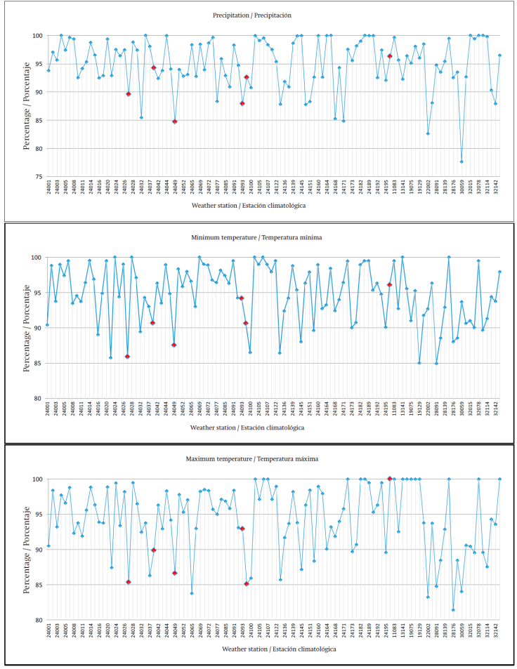
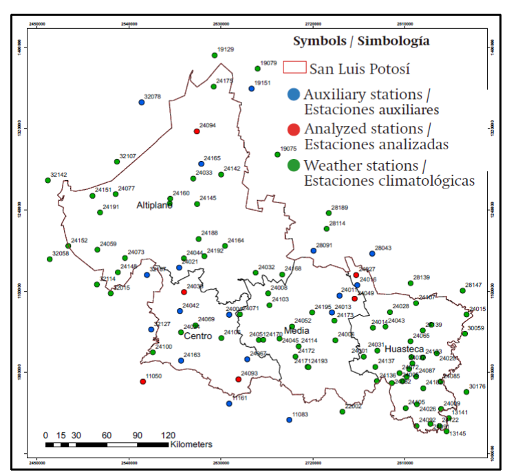
Figure 2 shows the location and distribution of the 108 weather stations. It also shows the analyzed and auxiliary stations, which served to define the best method for deducing the missing data.
Selection of weather stations
Six weather stations (Table 1), two in the Centro region, one from each of the other regions (Altiplano, Medio and Huasteca) and one of the stations bordering the state, were selected in order to delimit and represent the study area. In each of these 15 % of the precipitation (1,489 of 9,862 from 27 years) and 25 % of the maximum and minimum temperature (1,489 to 5,844 from 16 years) information was removed; later, in order to generate the missing data, records from the respective auxiliary stations corresponding to each analyzed station were used.
Table 1 Distance between the analyzed and auxiliary stations (km).
| Station | Auxiliary stations | |||
|---|---|---|---|---|
| Ocampo, Ocampo, Gto.: 11050 Distance (km) |
Pino Suarez, Zac.: 32127 52.34 |
Armadillo de los Infante, S. L. P.: 24004 107.5 |
El Vergel, San Luis de la Paz, Gto.: 11161 87.67 |
|
| El Salto, Cd. del Maíz, S. L. P.: 24027 Distance (km) |
Abritas, El Naranjo, S. L. P.: 24016 10.05 |
San Pablo, Tula, Tamps.: 28091 48.34 | La Boquilla, Ocampo, Tamps.: 28043 26.33 |
|
| Los Pilares, S. L. P.: 24038 Distance (km) |
Armadillo de los Infante, SLP: 24004 49.64 |
Mexquitic de Carmona, SLP: 24042 19.57 | El Grito, Moctezuma, S.L.P.: 24021 24.67 |
Espíritu Santo, Pinos, Zac.: 32187 40.86 |
| Papagayos, Cd. del Maíz, S. L. P.: 24049 Distance (km) |
Cd. Del Maíz, S. L. P.: 24011 15.68 |
Abritas, El Naranjo, S. L. P.: 24016 13.72 | Álvaro Obregón, Cd. del Maíz, S. L. P.: 24013 26.17 |
|
| Tierranueva, S. L. P.: 24093 Distance (km) |
Bledos, Villa de Reyes, S. L. P.: 24163 59.5 |
San José Alburquerque, Santa María del Rio, S. L. P.: 24067 21.56 | El Vergel, San Luis de la Paz, Gto.: 11161 26.02 |
Xichu, Gto.: 11083 64.02 |
| Vanegas, S. L. P.: 24094 Distance (km) |
San
Tiburcio, Mazapil, Zac.: 32078 61.78 |
Las Margaritas, Dr. Arroyo, N. L.: 19151 68.55 | San José
de Coronado, Real de Catorce, S. L. P.: 24165 68.55 |
|
Methods for estimating missing data
The methods used were: deductive rational (DR), proposed by Campos-Aranda (1998), which is determined from the values of the record itself, and normal ratio (NR) (Aparicio, 2007), represented in Equation 1.
where PX = missing precipitation at station x, Nx, Na, Nb,…Nn = average daily precipitation of the missing station (x) and the auxiliary stations a, b,…n (averages of all historical series) and Pa, Pb,…Pn = precipitation recorded at the auxiliary stations of the day where the datum is missing at station x.
The U.S. National Weather Service’s inverse square distance (ISD) method (Chow, Maidment, & Mays, 1996), represented in the following equation, was also used:
where: PX = lost datum at station x and Pi = existing datum at auxiliary station i, for which i = 1, 2,… n for the same day.
In Equation 3, Di = distance between each neighboring auxiliary station and station x where the lost datum is presented. Campos-Aranda (1998) recommend using four auxiliary stations (the nearest), so that each remains located in one of the quadrants that define the coordinate axes that pass through the incomplete station, generally north-south and east-west.
Statistical indices to evaluate the error estimate
Three statistical indices were used: the Willmott index of agreement (d) (Willmott, 1981), mean standard error or root mean square error (RMSE) (Rivas & Carmona, 2010) and the coefficient of determination (R2) (Cervantes-Osornio et al., 2013; Kelso-Bucio et al., 2012; Wright, 2001), which are defined as:
where R2 = coefficient of determination, ai = datum estimated by the method, ti = observed datum, N = number of observations or estimates, = average of the data estimated by the method and = average of the observed data.
If RMSE = 0 and R2 = d = 1, then there is a perfect fit. The results are excellent when d ≥ 0.95 and R2 > 0.80 (Cai et al., 2007; Ruiz-Álvarez, Arteaga-Ramírez, Vázquez-Peña, Ontiveros-Capurata, & López-López, 2012).
Results and discussion
Table 2 shows a summary of the statistical precipitation indices, and a better fit with the ISD method with an RMSE average of 38.7 mm is observed. The d values on average were 0.85, 0.68 and 0.68 for ISD, DR and NR, respectively, which have no values greater than 0.95 as recommended by Cai et al. (2007) and Ruiz-Álvarez et al. (2012); however, the ISD method shows a better fit.
Table 2 Statistical fit indices of the methods for estimating missing precipitation data records.
| Station | ISD | DR | NR | |||||
|---|---|---|---|---|---|---|---|---|
| RMSE | D | R2 | RMSE | d | RMSE | d | R2 | |
| Ocampo, Ocampo: 11050 | 19.503 | 0.917 | 0.144 | 41.672 | 0.556 | 32.254 | 0.865 | 0.166 |
| El Salto, Cd. del Maíz: 24027 | 73.682 | 0.911 | 0.216 | 84.242 | 0.861 | 80.477 | 0.926 | 0.376 |
| Los Pilares, San Luis Potosí :24038 | 21.004 | 0.890 | 0.363 | 29.509 | 0.672 | 71.649 | 0.587 | 0.271 |
| Papagayos, Cd. del Maíz: 24049 | 61.666 | 0.918 | 0.298 | 97.865 | 0.856 | 117.633 | 0.869 | 0.173 |
| Tierranueva: 24093 | 28.728 | 0.845 | 0.335 | 42.390 | 0.638 | 41.627 | 0.728 | 0.184 |
| Vanegas : 24094 | 27.870 | 0.615 | 0.030 | 24.206 | 0.485 | 78.453 | 0.129 | 0.012 |
| Average | 38.742 | 0.849 | 0.231 | 53.314 | 0.678 | 70.349 | 0.684 | 0.197 |
On the other hand, stations 11050, 24027, 24038, 24049 and 24093 show a lower RMSE value with ISD, compared with that obtained with DR and NR, while the data analyzed at station 24094, according to the RMSE statistic, indicate a lower error with the DR method.
In a study conducted in Colombia, Toro-Trujillo et al. (2015) report similar values among the statistical indices when analyzing the precipitation variable, but a better Willmott index of agreement (d) result with the ISD method is highlighted; therefore, they propose it as the best method for estimating missing data, a situation also presented in this study, since the best estimate was obtained with the ISD method. Moreover, considering that R2 averaged 0.231 and 0.197 for ISD and NR, respectively, it can be deduced that there is little strength in the linear relationship between the estimated and observed value, mainly because precipitation is a discrete variable with a high frequency of values close to zero.
Figure 3 illustrates the relationship between observed and estimated precipitation values, with the ISD and NR methods at weather stations 24027 El Salto, 24038 Los Pilares and 24049 Papagayos. The ISD method has, on average, a better fit of the estimated values with respect to the observed ones, which is consistent with the results obtained by Hubbard and You (2005), Eischeid, Pasteris, Diaz, Plantico, and Lott (2000) and You, Hubbard, and Goddard (2008). Moreover, Teegavarapu and Chandramouli (2005) mention that the ISD method better estimates the observed data, plus it can be used in any time period, i.e., in daily, monthly and annual data.
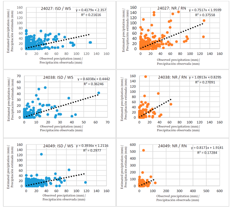
Figure 4 shows the relationship between the observed and estimated maximum temperature with the ISD and NR methods; similar behavior can be observed in the two methods, possibly because temperature is a more localized variable (Toro-Trujillo et al., 2015; You et al., 2008).
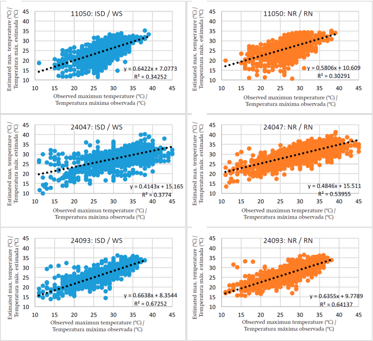
Table 3 shows the statistical indices calculated with the three described methods to determine which one estimates more accurately the missing maximum temperature data records. It also shows that the values are similar to one other, although the RMSE results are higher than those with the ISD method, followed by the DR and finally the NR methods. According to the Willmott index, the NR method has a better fit because, in general, it has a higher value at the stations, followed by the DR and ISD methods, respectively.
Table 3 Statistical fit indices of the methods for estimating missing maximum temperature data records.
| Station | ISD | DR | NR | |||||
|---|---|---|---|---|---|---|---|---|
| RMSE | D | R2 | RMSE | d | RMSE | d | R2 | |
| Ocampo, Ocampo: 11050 | 3.264 | 0.685 | 0.343 | 3.620 | 0.582 | 1.761 | 0.843 | 0.303 |
| El Salto, Cd. del Maíz: 24027 | 3.744 | 0.769 | 0.377 | 2.692 | 0.803 | 2.670 | 0.880 | 0.540 |
| Los Pilares, San Luis Potosí :24038 | 3.938 | 0.707 | 0.493 | 2.282 | 0.887 | 3.244 | 0.769 | 0.501 |
| Papagayos, Cd. del Maíz: 24049 | 2.823 | 0.751 | 0.251 | 2.177 | 0.845 | 1.816 | 0.864 | 0.285 |
| Tierranueva: 24093 | 1.277 | 0.937 | 0.673 | 1.933 | 0.888 | 1.133 | 0.952 | 0.641 |
| Vanegas : 24094 | 2.905 | 0.801 | 0.467 | 2.194 | 0.891 | 1.938 | 0.897 | 0.463 |
| Average | 2.992 | 0.780 | 0.434 | 2.150 | 0.866 | 2.094 | 0.867 | 0.455 |
At stations 11050, 24038, 24049 and 24093, the coefficient of determination R2 is greater with the ISD method, and with the others it is greater with NR, although the R2 are very similar. Campos-Aranda (2005) recommends against using low linear relationship methods if the coefficients of determination do not have values greater than 0.8; therefore, because the present study presents a low linear relationship, it is advisable to use either the ISD or NR methods, since they have similar statistics.
Figure 5 compares the observed and estimated minimum temperature with the ISD and NR methods, at the stations studied.
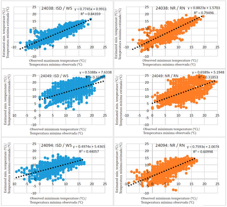
Table 4 shows the statistics that allow identifying the method that has the best fit to the minimum temperature data. The Willmott index is higher with DR at stations 24027, 24049 and 24094, with NR at 11050 and 24038, and with ISD at 24093. It also shows that the d value varies in a very similar way in the three methods. Stations 24027, 24049 and 24094 reflected lower RMSE values with the DR method, whereas 24038 and 24093 did so with the ISD method, and 11050 with the NR method.
Table 4 Statistical fit indices of the methods for estimating missing minimum temperature data records.
| Station | ISD | DR | NR | |||||
|---|---|---|---|---|---|---|---|---|
| RMSE | d | R2 | RMSE | D | RMSE | d | R2 | |
| Ocampo, Ocampo: 11050 | 1.019 | 0.975 | 0.794 | 1.031 | 0.968 | 0.944 | 0.978 | 0.764 |
| El Salto, Cd. del Maíz: 24027 | 3.097 | 0.849 | 0.447 | 1.921 | 0.948 | 1.979 | 0.944 | 0.706 |
| Los Pilares, San Luis Potosí: 24038 | 1.450 | 0.967 | 0.844 | 1.578 | 0.962 | 1.494 | 0.970 | 0.795 |
| Papagayos, Cd. del Maíz: 24049 | 3.710 | 0.761 | 0.327 | 2.661 | 0.854 | 4.110 | 0.755 | 0.319 |
| Tierranueva: 24093 | 1.261 | 0.969 | 0.810 | 1.833 | 0.942 | 2.275 | 0.925 | 0.711 |
| Vanegas : 24094 | 3.307 | 0.801 | 0.441 | 1.569 | 0.960 | 1.829 | 0.947 | 0.610 |
| Average | 2.318 | 0.887 | 0.611 | 1.766 | 0.939 | 2.105 | 0.920 | 0.651 |
Conclusions
The methods used to estimate the missing precipitation data records allowed identifying the one which best estimates the results, and according to the statistical indicators it is the ISD method; therefore, for precipitation, this is the best alternative when data are available for the same period at auxiliary stations. The results obtained by analyzing the maximum and minimum temperature data indicate little variability among methods, as the calculated data are similar to those observed; therefore, both the behavior and errors are very similar with all three methods. Accordingly, the U.S. National Weather Service’s inverse square distance (ISF) method is an efficient alternative for completing missing data records in a continuous series; therefore, it was the method used to estimate missing data at 108 weather stations in the state of San Luis Potosí.

