


Services on Demand
Journal
Article
 text in
  English (pdf)
 Article in xml format
 Article references
 Send this article by e-mail
Indicators
-
 Cited by SciELO
 -
 Access statistics
Related links
-
 Similars in
SciELO
Similars in
SciELO
Share

 Permalink
Tecnología y ciencias del agua
On-line version ISSN 2007-2422
Tecnol. cienc. agua vol.10 n.5 Jiutepec Sep./Oct. 2019 Epub Feb 15, 2020
https://doi.org/10.24850/j-tyca-2019-05-02
Articles
Best PDF in 19 large annual series of MDP from the San Luis Potosi state, Mexico.
1Profesor jubilado de la Universidad Autónoma de San Luis Potosí, México, campos_aranda@hotmail.com
All hydraulic works are planned and designed based on Floods Design. Without hydrometric information, these predictions are estimated using hydrological methods that yield the sought flows by means of design rainfalls. Design rainfall is estimated based on pluviometer records of annual maximum daily precipitation (MDP) due to the shortage of pluviographs. The probabilistic analysis of the annual MDP series is identical to that of the floods; however, neither adequate probability distribution functions (PDFs) nor those that should be applied by precept have been defined so far, hence the need to try several. First, the best PDF was searched for using the L-ratio diagram, which includes six models with three fit parameters. An objective selection is made by using the weighted absolute distance, in the 19 annual MDP records with more than 50 data from the state of San Luis Potosi, Mexico. Then eight descriptive ability (DA) indexes are described and applied to the eight PDFs that were compared, in each of the 19 PMD records. The results are concentrated and analyzed for geographic areas of the state: Potosino Plateau and Middle Zone. Results show that Wakeby PDF is a model having high DA and for that reason, its application is suggested as precept. The two best PDF options are also highlighted in each of the 19 records processed, according to the eight DA indexes. Finally, a comparison of predictions with periods of return of 50, 100, 500 and 1000 years is carried out to explore shallowly the predictive ability of the PDFs found as best options. In each registry four PDFs are applied, the one obtained according to the L-ratio diagram; the two best PDFs according to the eight DA indices and the Wakeby distribution. It is concluded that the use of the L-ratio diagram and the application of the eight DA indexes are adequate and lead to a good approximation, since it was not difficult to select the adopted predictions, besides the similarity of the predictions calculated in each register promotes confidence in such estimations.
Keywords: L-ratio diagram; standard error of fit; relative standard error of fit; mean absolute error; maximum absolute error; Akaike information criterion; Q-Q correlation coefficient; concordance indexes and predictive ability
Todas las obras hidráulicas se planean y diseñan con base en las crecientes de diseño. Sin información hidrométrica, estas predicciones se estiman con métodos hidrológicos que transforman lluvias de diseño en los gastos buscados. La escasez de pluviógrafos origina que las lluvias de diseño se estimen a partir de los registros de precipitación máxima diaria (PMD) anual de los pluviómetros. El análisis probabilístico de las series de PMD anual es idéntico al de las crecientes; pero aún no se han definido funciones de distribución de probabilidades (FDP) adecuadas o que se deban aplicar bajo precepto, por lo cual es necesario probar varias. Primero se buscó la mejor FDP en el diagrama de cocientes L, que incluye seis modelos de tres parámetros de ajuste. Se realiza una selección objetiva al emplear la distancia absoluta ponderada en los 19 registros de PMD anual con más de 50 datos del estado de San Luis Potosí, México. Después se describen y aplican ocho índices de habilidad descriptiva (HD) a las ocho FDP que fueron contrastadas en cada uno de los 19 registros de PMD. Los resultados se concentran y analizan por áreas geográficas del estado: Altiplano Potosino y Zona Media. Se obtuvo que la FDP Wakeby es un modelo de gran HD y por ello se sugiere que su aplicación se realice bajo precepto. También se definen las dos mejores opciones de FDP en cada uno de los 19 registros procesados de acuerdo con los ocho índices de HD. Por último, se realiza un contraste de predicciones con periodos de retorno de 50, 100, 500 y 1000 años, para explorar de manera somera la habilidad predictiva de las FDP encontradas como mejores opciones. En cada registro se aplican cuatro FDP: la obtenida según el diagrama de cocientes L, las dos mejores FDP según los ocho índices de HD y la distribución Wakeby. Se concluye que el uso del diagrama de cocientes L y la aplicación de los ocho índices de HD son adecuados y conducen a una buena aproximación, pues no se tuvo dificultad para seleccionar las predicciones adoptadas y la similitud que mostraron estas estimaciones en cada registro genera confianza en tales estimaciones.
Palabras clave: diagrama de cocientes L; error estándar de ajuste; error relativo estándar de ajuste; error absoluto medio; error absoluto máximo; criterio de información de Akaike; coeficiente de correlación de Q-Q; índices de concordancia y habilidad predictiva
Introduction
The Design Floods hydrologically size all the hydraulic works, in the different stages that they cross. In sites of interest and their respective basins, which do not have annual maximum flow information, the Design Floods must be estimated based on hydrological methods that transform a design rainfall into the response hydrograph or the sought peak flow (Mujumdar & Nagesh-Kumar, 2012). Design rainfalls come from the Intensity-Duration-Frequency (IDF) curves that characterize the way it rains in the study area. The shortage of rainfall recorders prevents the construction of the IDF curves and therefore its estimation is used, based on the available records of the pluviometric or rain-gauge stations of wider coverage and larger records (Teegavarapu, 2012; Johnson & Sharma, 2017).
The annual maximum daily precipitation records (PMD, for its Spanish initials) are probabilistically processed in an identical way as those of annual maximum flow or floods; going through four stages: (1) search for records, including debugging and verification of their homogeneity; (2) choice of a cumulative probability distribution function or FDP (for its Spanish initials), that is, of the probabilistic model that will allow obtaining the predictions associated with low probabilities of exceedance; (3) application of one or more methods of estimation of the fit parameters of FDP and (4) validation of the adopted FDP and its predictions Rao & Hamed, 2000; Meylan, Favre, & Musy, 2012; Stedinger, 2017).
The objective of the study was to select the best FDPs, which should be applied in the probabilistic analysis of annual PMD series. First, the L-ratio diagram is exposed and applied through the weighted absolute distance to objectively adopt the best FDP of the six that it includes. Then, an approach based on eight descriptive ability indexes for selection is followed, among the eight FDPs that are contrasted. The concentrated results of the Potosino Plateau and Middle Zone of the state of San Luis Potosí, Mexico, are exposed and analyzed, in which 9 and 10 annual PMD records were processed, with 50 or more data. Finally, a contrast of predictions with return periods of 50, 100, 500 and 1000 years is made and conclusions are drawn regarding the predictive capacity of the selected FDPs.
Data of PMD processed
Debugged series
Based on the Excel file updated until 2015 of the San Luis Potosí weather stations, provided to the author by the Local Office of the National Water Commission (Conagua), all records of annual maximum daily precipitation (PMD) were selected with more than 40 values and scarce missing data, 100 series were obtained (Campos-Aranda, 2018). Then a ratification of their minimum and maximum extreme values was carried out with the aid of CONAGUA, to obtain the so-called debugged series.
Homogeneity tests applied
The Neumann Von Test was applied to each debugged series as a general test, which detects non-randomness by deterministic components unspecified and several specific tests: Anderson and Sneyers of persistence, Kendall and Spearman of trend, Bartlett of inconsistency in dispersion and Cramer of changes in the mean. These tests can be found in WMO (1971), and Machiwal and Jha (2008). It was found that a total of 39 series were random or not, or they presented persistence and/or trend.
Series to be processed
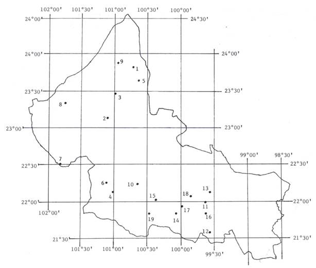
The 39 non-homogeneous series were eliminated, as well as those with less than 50 data; with these restrictions, 35 records of annual PMD were available in the state of San Luis Potosí. Nine series belong to the Potosino Plateau (AP), ten to the middle zone (ZM) and 16 to the Huasteca Region. In this study the 19 series that are located in the arid and semi-arid climates of the geographical areas AP and ZM, whose altitudes are generally higher than one thousand meters, were processed. Table 1 shows their altitude, record width, statistical values and L-moment ratios (Equations (6) to (8)). The first nive climatological stations belong to the AP and the 10 remaining to the ZM. Figure 1 shows their geographical location in the state of San Luis Potosí; Mexico.
Table 1 Altitude, record width and minimum and maximum values of the 19 annual maximum daily precipitation series (PMD) of the state of San Luis Potosí, Mexico.
| No. | Station name | Altitude (masl1) |
Record | PMD | ||
|---|---|---|---|---|---|---|
| Period | n 2 | min | Max | |||
| 1 | Cedral | 1702 | 1946-2014 | 66 | 19.0 | 315.8 |
| 2 | Charcas | 2126 | 1961-2014 | 54 | 12.0 | 117.0 |
| 3 | La Maroma | 1900 | 1965-2014 | 50 | 16.0 | 140.1 |
| 4 | Los Filtros (SLP) | 1904 | 1949-2014 | 66 | 15.9 | 111.0 |
| 5 | Matehuala | 1630 | 1961-2014 | 54 | 25.5 | 200.0 |
| 6 | Mexquitic | 1749 | 1943-2014 | 72 | 12.0 | 107.0 |
| 7 | Peñón Blanco | 2099 | 1950-2014 | 57 | 13.0 | 235.0 |
| 8 | Santo Domingo | 1415 | 1961-2013 | 52 | 19.0 | 270.0 |
| 9 | Vanegas | 1746 | 1964-2013 | 50 | 12.0 | 90.0 |
| 10 | Armadillo de los Infante | 1636 | 1961-2013 | 52 | 22.0 | 133.0 |
| 11 | Cárdenas | 1353 | 1946-2013 | 61 | 21.5 | 180.5 |
| 12 | Lagunillas | 908 | 1954-2013 | 53 | 30.0 | 210.0 |
| 13 | Ojo de Agua | 1148 | 1960-2013 | 52 | 45.0 | 300.2 |
| 14 | Ojo de Agua Seco | 1077 | 1961-2013 | 51 | 26.5 | 172.5 |
| 15 | Paso de San Antonio | 1246 | 1958-2013 | 52 | 26.0 | 200.0 |
| 16 | Rayón | 1258 | 1961-2013 | 51 | 33.5 | 330.0 |
| 17 | Río Verde | 987 | 1961-2013 | 52 | 27.0 | 126.3 |
| 18 | San Francisco | 1066 | 1961-2013 | 50 | 12.0 | 135.0 |
| 19 | San José Alburquerque | 1863 | 1961-2014 | 50 | 21.0 | 126.5 |
L-ratio diagram
L-moments of the sample
L-moments are linear combinations of the moments of weighted probability (b
r
), for that reason they are robust before the dispersed values of sample. Their calculation begins by ordering the available series (x
i
) of annual PMD from lowest to highest (
In the previous expression the order number r varies from 0 to 3 and n is the data number of the annual PMD series. It follows that b 0 is equal to the arithmetic mean. The L-moments of the sample (l) and their respective quotients (t) of similarity with the coefficients of variation, asymmetry and kurtosis are:
L-ratio diagram
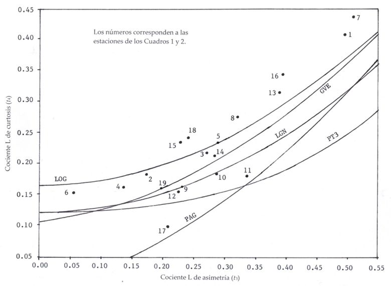
It has on the abscissa axis t 3 and on the ordinate t 4. The FDPs of three fit parameters are curved lines with the following polynomial-type equations (Hosking & Wallis, 1997):
Generalized Logistics (LOG):
Generalized Pareto (PAG):
Log-Normal (LGN):
Pearson type III (PT3):
and General of Extreme Values (GVE):
being:
Using the logarithms of the data in Equations 1 to 8, the logarithmic L- ratios are obtained and then the expression 12 can be used to evaluate the FDP Log-Pearson type III. Figure 2 shows a portion of the L-moments ratio diagram from Hosking and Wallis (1997).
Absolute weighted distance
One of the recent approaches to choose the best FDP, at the local and regional level, consists of taking to the L-ratio diagram the values of the sample (t 3 and t 4) and defining its proximity to any of the curves, in order to obtain the best probabilistic model. This is relatively simple in local analyses, but it is complicated in the regional approach as pointed out by Peel, Wang, Vogel and McMahon (2001), since then there is a cloud of points. To avoid subjectivity in the selection of the FDP, it has been proposed to evaluate the Absolute Weighted Distance (DAP) with the following expression (Yue & Hashino, 2007):
where NE is the number of stations that make up the region, n
j
is the data number of each PMD record,
Distribution functions to be contrasted
Based on the L-ratio diagram, six FDP can be tested and as accepted a priori to eliminate the one that was not selected at least once (see Table 3) in the 19 annual PMD records to be processed, the Pearson Type III distribution was not contrasted and then the LOG, PAG, LGN, GVE and LP3 models will be tested.
Table 2 Statistical parameters and L-moment ratios of the 19 series of annual maximum daily precipitation (PMD) of the state of San Luis Potosí, Mexico.
| Sta. No. |
Statistical parameters3 | L-moment ratios4 | ||||||
|---|---|---|---|---|---|---|---|---|
|
|
l 2 | S | Cs | t 3 | t 4 |
|
|
|
| 1 | 47.1 | 13.465 | 38.6 | 5.501 | 0.49274 | 0.41041 | 0.20245 | 0.20806 |
| 2 | 48.8 | 12.068 | 22.0 | 0.974 | 0.17331 | 0.18124 | -0.06888 | 0.17927 |
| 3 | 46.6 | 10.807 | 21.3 | 2.006 | 0.27042 | 0.21953 | 0.05484 | 0.16449 |
| 4 | 43.0 | 8.448 | 15.7 | 1.315 | 0.13515 | 0.16117 | -0.04764 | 0.13773 |
| 5 | 59.3 | 14.243 | 29.2 | 2.471 | 0.28588 | 0.23605 | 0.06420 | 0.13996 |
| 6 | 47.8 | 9.521 | 17.1 | 0.540 | 0.05475 | 0.15489 | -0.14445 | 0.17245 |
| 7 | 47.8 | 15.395 | 40.2 | 3.669 | 0.51286 | 0.44109 | 0.19048 | 0.26367 |
| 8 | 57.6 | 16.564 | 37.8 | 3.685 | 0.31725 | 0.27714 | 0.02817 | 0.14591 |
| 9 | 37.6 | 10.013 | 18.4 | 1.028 | 0.22725 | 0.16424 | -0.00150 | 0.14389 |
| 10 | 57.5 | 14.504 | 27.3 | 1.287 | 0.28601 | 0.18574 | 0.08089 | 0.14044 |
| 11 | 67.7 | 20.216 | 38.9 | 1.457 | 0.33709 | 0.18138 | 0.11049 | 0.12095 |
| 12 | 77.8 | 18.480 | 35.0 | 1.525 | 0.22455 | 0.15699 | 0.02475 | 0.10105 |
| 13 | 91.4 | 21.459 | 46.5 | 2.586 | 0.38619 | 0.31739 | 0.16556 | 0.20467 |
| 14 | 69.3 | 14.883 | 28.9 | 1.694 | 0.28166 | 0.21420 | 0.08873 | 0.16202 |
| 15 | 69.3 | 13.793 | 27.6 | 2.219 | 0.22726 | 0.23726 | 0.01936 | 0.18991 |
| 16 | 76.4 | 19.343 | 45.5 | 3.765 | 0.39215 | 0.34343 | 0.13435 | 0.21192 |
| 17 | 58.4 | 12.973 | 23.4 | 0.934 | 0.20926 | 0.09728 | 0.05010 | 0.06390 |
| 18 | 46.7 | 12.757 | 24.4 | 1.461 | 0.23966 | 0.24363 | -0.03897 | 0.21540 |
| 19 | 50.1 | 11.466 | 21.7 | 1.434 | 0.19616 | 0.16114 | 0.00396 | 0.08689 |
Symbols:
1meters above sea level.
2number of processed data.
3
l1, l2L moments of order 1 and 2.
Sstandard deviation, in millimeters.
Cscoefficient of asymmetry, dimensionless.
4t 3asymmetry L-ratio, dimensionless.
t4kurtosis L-ratio, dimensionless.
Table 3 Three minimum values of the DAP and their respective PDFs of the L-moment ratio diagram, in the 19 series of annual PMD processed from the state of San Luis Potosí, Mexico.
| No. | Station | DAP and FDP | ||
|---|---|---|---|---|
| 1st option | 2nd option | 3rd option | ||
| 1 | Cedral | 0.0414 | 0.0511 | 0.0717 |
| LOG | GVE | LP3 | ||
| 2 | Charcas | 0.0105 | 0.0299 | 0.0350 |
| LOG | GVE | LGN | ||
| 3 | La Maroma | 0.0081 | 0.0218 | 0.0394 |
| LOG | GVE | LGN | ||
| 4 | Los Filtros (SLP) | 0.0146 | 0.0207 | 0.0238 |
| LP3 | LOG | GVE | ||
| 5 | Matehuala | 0.0013 | 0.0163 | 0.0296 |
| LOG | LP3 | GVE | ||
| 6 | Mexquitic | 0.0143 | 0.0297 | 0.0316 |
| LOG | LGN | PT3 | ||
| 7 | Peñón Blanco | 0.0552 | 0.0635 | 0.1078 |
| LOG | GVE | LGN | ||
| 8 | Santo Domingo | 0.0233 | 0.0266 | 0.0517 |
| LP3 | LOG | GVE | ||
| 9 | Vanegas | 0.0011 | 0.0110 | 0.0215 |
| LGN | GVE | LP3 | ||
| 10 | Armadillo de los Infante | 0.0012 | 0.0160 | 0.0208 |
| LGN | LP3 | GVE | ||
| 11 | Cárdenas | 0.0053 | 0.0115 | 0.0132 |
| LP3 | PAG | PT3 | ||
| 12 | Lagunillas | 0.0052 | 0.0169 | 0.0170 |
| LGN | GVE | PT3 | ||
| 13 | Ojo de Agua | 0.0264 | 0.0450 | 0.0733 |
| LOG | GVE | LP3 | ||
| 14 | Ojo de Agua Seco | 0.0102 | 0.0186 | 0.0292 |
| GVE | LOG | LGN | ||
| 15 | Paso de San Antonio | 0.0276 | 0.0620 | 0.0674 |
| LOG | GVE | LP3 | ||
| 16 | Rayón | 0.0486 | 0.0666 | 0.0838 |
| LOG | GVE | LP3 | ||
| 17 | Río Verde | 0.0148 | 0.0401 | 0.0593 |
| PAG | PT3 | LP3 | ||
| 18 | San Francisco | 0.0291 | 0.0622 | 0.0759 |
| LOG | GVE | LGN | ||
| 19 | San José Alburquerque | 0.0002 | 0.0083 | 0.0258 |
| GVE | LGN | PT3 | ||
The eight FDPs that were contrasted include the Beta Kappa and Beta Pareto models proposed by Mielke and Johnson (1974) that are not popular in Mexico, but that were compared in a pioneering work of optimal selection of distributions with three fitting parameters in records of annual PMD, that of Wilks (1993), with good results for Beta-κ (BEK) in series of maximums and values above a threshold for Beta-P (BEP): Nguyen, El Outayek, Lim, and Nguyen (2017) also include them in their contrast.
Finally, the FDP Wakeby (WAK) was included, which has five fit parameters, it was proposed by Houghton (1978) and allows the left and right ends of the sample to be modeled separately. Nguyen et al. (2017) find that the Wakeby distribution is the best in descriptive ability.
To avoid more variables involved in the selection of the best FDPs, in models that have several estimation methods of their fit parameters, the L-moments method was exclusively applied, which has proven to be consistent and accurate. Such method in the GVE, LOG and PAG models is not exposed, since it has been described in several articles by the author, for example in Campos-Aranda (2015; 2016). It can also be consulted in Hosking and Wallis (1997), Rao and Hamed (2000) and Stedinger (2017). The FDPs Log-Normal (LGN) and Wakeby (WAK) were fitted with the L-moments method described by Hosking and Wallis (1997).
Regarding the Log-Pearson type III distribution (LP3) it was fitted with the moments method, in the logarithmic and real domains (WRC, 1977; Bobée & Ashkar, 1991; Campos-Aranda, 2002), selecting that of lower standard error of fit (Kite, 1977). The Beta distributions were fitted with the iterative method of maximum likelihood of Mielke and Johnson (1974), adopting as initial value of the scale parameter the mean of the PMD record and of the shape parameter a value of five. The maximum of iterations was taken to two thousand.
Descriptive ability indexes
Diagnostic Graphics
The P-P and Q-Q graphs of empirical versus calculated probability and observed versus estimated quantity have become popular (Coles, 2001; Wilks, 2011) and are a simple and effective way to compare the results of a FDP contrasted. Their disadvantage lies in the subjective appreciation that is made when comparing various FDPs, with such graphs, since a numerical value is not available (Nguyen et al., 2017). Campos-Aranda (2015) has exposed such graphs and visualizes more useful the Q-Q graph, to observe predictions overestimated (for being above the line at 45°) or underestimated (for being below the line at 45°).
Statistical tests
These tests, like the Chi-square, the Kolmogorov-Smirnov or Anderson-Darling, can justify that a sample can be accepted coming from a specific distribution that is analyzed. In the first two tests, their disadvantage lies in having low power and in the second, only being applicable for a specific FDP (Meylan et al., 2012).
Goodness-of-fit indexes
They have the advantage of being of easy calculation and commonly involve the difference between the observed values x
i
and those estimated with the FDP that is contrasted
Empirical probability formula
Meylan et al. (2012) indicate that all the empirical equations that assign probabilities are based on ordering the available sample or series in upward magnitudes, making it possible to associate an order i with each datum and then make use of the following general formula, which ensures symmetry with respect to the median:
in which, c is a constant quantity and n is the size of the record or series of the annual PMD.
Haktanir (1991) describes a practical finding of 1971 by J.R. Stipp and G.K. Young who processed 37 annual flood records of exactly 20 data each, all in the USA. They estimated the probability of each maximum and minimum event of each series based on the Log-Pearson type III distribution and then equated those values with the one obtained from the Equation 15, finding that c had an approximate magnitude of 0.40, whereby:
Haktanir (1991) also points out that years later, Cunnane arrives at the same Equation 16 in a theoretical and independent way, stating that such formula is not specific of a FDP and that their results are unbiased and have a minimum square error. Cunnane (1978) also finds, with statistical arguments, that the popular Weibull formula (Benson, 1962) is only applicable for a uniform distribution, so it is not convenient to use it in series of extreme hydrological values (floods, droughts, PMD, etc.).
Standard error of fit (EEA)
It is the most common index (Chai & Draxler, 2014), it was established in the mid-seventies (Kite, 1977) and has been applied in Mexico using the empirical formula of Weibull (Benson, 1962). Now it will be applied using the Cunnane formula (Equation 16), which according to Stedinger (2017) leads to probabilities of non-exceedance (
in which, x
i
are the observed data ordered from lowest to highest,
Relative standard error of fit (EREA)
In the EEA all the differences or residuals are squared and this implies giving greater weight to the high values of the sample, to reduce this impact the EREA is applied, which is dimensionless, its equation is (Pandey & Nguyen, 1999; Nguyen et al., 2017):
Mean Absolute Error (EAM)
Its advantages lie in having the units of the variable, like the EEA, and avoiding that the impact of the scattered values be squared and therefore EEA ≥ EAM (Willmott & Matsuura, 2005). Its expression is (Pandey & Nguyen, 1999; Nguyen et al., 2017):
Maximum Absolute Error (EAMx)
This index shows the largest of the errors or absolute residuals, for that reason Nguyen et al. (2017) have indicated that it is related to the statistics of the Kolmogorov-Smirnov test; its equation is:
Akaike Information Criterion (AIC)
This index uses in its original conception the maximum value reached in the likelihood function during the fit, with such method, of the FDP that is contrasted. In order to apply such index, Nguyen et al. (2017) use the sum of squared errors (SEC) as indictor of the fitting quality and then its equation is:
In these first five indexes, the lowest value of them indicates the best fit of FDP and its maximum magnitude the worst fit of such contrasted FDP. In the following three indexes occurs the opposite, so that a maximum value indicates a good fit of the FDP and vice versa.
Q-Q Correlation Coefficient (COC)
This index has been used as the main selection criterion by Zalina et al. (2002), it indicates the linear dependence that exists in the Q-Q graph; whereby, it varies from zero to one. The values of the COC close to the unit indicate a good fit of the FDP that is contrasted; its equation is:
where,
Concordance indexes (d1, d2)
According to Legates and McCabe (1999), Willmott pointed out since the beginning of the eighties that the COC index is limited and insensitive to the differences and variances between x
i
and
The numerator is the SEC and the denominator is called the potential error, because it is the maximum value that the difference between x
i
and
As d 2 as d 1 vary from zero to one, with an interpretation equal to COC; usually, d 2 ≥ d 1.
Review of predictive ability
Available approaches
The predictive ability of the FDPs is related to the predictions made to return periods (Tr) higher than the size of the record (n), or to the comparison with the extreme values observed in the record. There are three approaches to test or verify such predictive ability, the first is the simplest and consists of the numerical contrast of the predictions obtained with each FDP for various adopted Tr.
The second approach of verification of predictive ability was exemplified by Haktanir (1992), he uses random samples generated with basic models (LP3, GVE and WAK), which use the fit parameters obtained in the records adopted as representative of the geographical regions studied. The best FDPs are adopted based on the lowest EREA.
From the decade of the nineties (Wilks, 1993; Zalina et al., 2002; Nguyen et al., 2017) a third approach of contrast has been proposed, based on random samples generated from the historical record, by sampling with replacement (bootstrap technique), which contrasts predictions within the record obtained with the tested FDPs, with the extreme values of such sample. The best FDPs are those that show less dispersion.
Adopted approach
It corresponds to the first and simplest, since it has the best FDP of each annual PMD record, according to the L-rates diagram and according to the eight indexes of descriptive ability applied. It consists of adopting one of the contrasted FDPs and their predictions, following a rule established a priori, for example, adopting the most critical or major values in most of the contrasted Tr; as long as such predictions are similar, which implies accuracy and generates confidence in the magnitudes adopted under such a subjective scheme.
Results according to the L-ratio Diagram
The evaluation of the Weighted Absolute Distance (Equation (14)) in each of the six FDPs of the L moment-ratio diagram (Equations (9) to (13)), making use of the values in Table 2, provided the three minimum values shown in Table 3, thus defining the best FDP and the subsequent two at local level of each series of annual PMD. In Figure 2 the values of t
3 and t
4 of each record, taken from Table 1, have been indicated. Most of these points define their proximity to an FDP, except for the stations: Los Filtros (No. 4), Santo Domingo (No 8) and Cárdenas (No. 11), with proximity to the LP3 model due to its values of
According to the summary by geographical areas of Table 4, it is concluded that the first or best option of FDP is the Generalized Logistics (LOG) with 10 selections, followed by the Log-Normal (LGN) and the Log-Pearson type III (LP3) with 3 selections and the least suitable one was the Pearson Type III (PT3) with no selection.
Table 4 Counting of the best selection of each FDP of the L-ratio diagram, in the 19 series of annual PMD of the state of San Luis Potosí, Mexico.
| FDP | Potosino Plateau | Middle Zone | Sums |
|---|---|---|---|
| Logística Generalizada (LOG) | 6 | 4 | 10 |
| Log-Normal (LGN) | 1 | 2 | 3 |
| Log-Pearson tipo III (LP3) | 2 | 1 | 3 |
| General de Valores Extremos (GVE) | 0 | 2 | 2 |
| Pareto Generalizada (PAG) | 0 | 1 | 1 |
| Pearson tipo III (PT3) | 0 | 0 | 0 |
| Sums | 9 | 10 | 19 |
Results according to descriptive ability
General observations
Regarding the Log-Pearson type III (LP3) distribution, a lower standard error of fit was obtained in the real domain in the Charcas, Los Filtros, Mexquitic and Santo Domingo stations of the Potosino Plateau and in the Paso de San Antonio and San Francisco stations from the Middle Zone. In the remaining 13 stations, the best fit was obtained in the logarithmic domain.
In relation to the Wakeby distribution (WAK), in a total of nine records it was obtained that the location parameter (ξ) was slightly higher than the minimum value of the series, which is strictly incorrect. In these nine records, the Wakeby distribution was fitted with ξ = 0, according to the procedure of Hosking and Wallis (1997) and its results (descriptive ability and predictions indexes) were compared against the previous fits. Only in the San José Alburquerque station it was found more adequate according to the EAMx and COC indexes, as well as less dispersed predictions, that is, it improved its predictive ability.
Results in the Potosino Plateau
Concentrate of numerical indexes
The three characteristic values (minimum, medium and maximum) of each index of descriptive ability (HD) obtained with each of the eight contrasting FDPs in the 9 rain-gauge stations of the Potosino Plateau of the state of San Luis Potosí, Mexico, have been concentrated in Table 4. Table 5 summarizes the eight unexposed tabulations of the results of each index with the eight FDPs contrasted in the 9 annual PMD records of the Potosino Plateau. Exclusively for the mean values, the best respective index value is indicated with circular parenthesis, pointing out such magnitude the best PDF at regional level. The worst indexes at regional level are also marked with rectangular parenthesis.
Table 5 Characteristic values of the eight descriptive ability (HD) indexes in the 9 series of annual PMD processed in the Potosino Plateau of the state of San Luis Potosí, Mexico.
| DA Index | FDP contrasted | |||||||
|---|---|---|---|---|---|---|---|---|
| BEK | BEP | LGN | GVE | LOG | PAG | LP3 | WAK | |
| EEA mín | 2.46 | 1.85 | 2.10 | 2.32 | 1.67 | 2.74 | 2.25 | 1.45 |
| EEA med | 8.13 | 7.19 | 7.10 | 6.98 | (6.37) | [8.35] | 6.54 | 7.06 |
| EEA máx | 20.40 | 16.42 | 15.68 | 14.85 | 14.80 | 15.96 | 13.40 | 15.73 |
| EREA mín | 0.041 | 0.038 | 0.033 | 0.035 | 0.041 | 0.073 | 0.048 | 0.040 |
| EREA med | 0.066 | (0.060) | 0.069 | 0.065 | 0.065 | [0.108] | 0.078 | 0.065 |
| EREA máx | 0.125 | 0.110 | 0.149 | 0.124 | 0.122 | 0.156 | 0.138 | 0.131 |
| EAM mín | 1.473 | 1.227 | 1.268 | 1.364 | 1.182 | 2.334 | 1.650 | 1.397 |
| EAM med | 3.107 | 2.669 | 3.013 | 2.802 | 2.618 | [3.886] | 3.127 | (2.555) |
| EAM máx | 6.705 | 5.409 | 5.498 | 4.978 | 4.920 | 6.737 | 6.989 | 5.106 |
| EAMx mín | 9.6 | 7.8 | 7.4 | 5.3 | 6.6 | 2.9 | 7.7 | 5.4 |
| EAMx med | 50.5 | 46.9 | 46.1 | 45.3 | 43.4 | [52.5] | (39.7) | 45.3 |
| EAMx máx | 161.2 | 129.5 | 120.2 | 116.0 | 116.1 | 122.8 | 100.5 | 115.4 |
| AIC mín | 311.5 | 302.2 | 302.2 | 313.8 | 309.7 | 300.0 | 306.4 | 293.6 |
| AIC med | 441.9 | 426.1 | 430.5 | 432.0 | (421.8) | [463.5] | 424.9 | 423.1 |
| AIC máx | 678.2 | 649.5 | 643.4 | 636.2 | 635.8 | 645.7 | 620.7 | 639.2 |
| COC mín | 0.916 | 0.944 | 0.935 | 0.945 | 0.953 | 0.914 | 0.938 | 0.951 |
| COC med | 0.971 | 0.976 | 0.972 | 0.975 | 0.978 | [0.959] | 0.976 | (0.980) |
| COC máx | 0.997 | 0.995 | 0.996 | 0.996 | 0.995 | 0.989 | 0.995 | 0.997 |
| d2 mín | 0.889 | 0.937 | 0.946 | 0.951 | 0.951 | 0.943 | 0.963 | 0.944 |
| d2 med | [0.967] | 0.979 | 0.981 | 0.982 | 0.983 | 0.974 | (0.985) | 0.980 |
| d 2 máx | 0.997 | 0.997 | 0.998 | 0.997 | 0.997 | 0.995 | 0.997 | 0.998 |
| d1 mín | 0.839 | 0.874 | 0.879 | 0.890 | 0.888 | 0.864 | 0.864 | 0.886 |
| d1 med | 0.913 | 0.927 | 0.921 | 0.925 | 0.929 | [0.897] | 0.918 | (0.933) |
| d1 máx | 0.956 | 0.957 | 0.953 | 0.951 | 0.957 | 0.923 | 0.952 | 0.965 |
Concentrate by rain-gauge stations
In Table 6, the results of the last columns of each tabulation not exposed of the analyzed index are integrated, that is, the best FDPs are obtained in each station according to each index. When two or more FDP showed equal value for the index analyzed at a certain station, the best FDP was chosen based on the best average value (last line of each tabulation not exposed).
Table 6 Best FDP according descriptive ability indexes in the 9 series of annual PMD processed of the Potosino Plateau of the state of San Luis Potosí, Mexico.
| Station | Descriptive ability indexes | Best two FDP* |
|||||||
|---|---|---|---|---|---|---|---|---|---|
| EEA | EREA | EAM | EAMx | AIC | COC | d2 | d1 | ||
| Cedral | LP3 | WAK | WAK | LP3 | LP3 | WAK | LP3 | WAK | WAK(4),LP3(4) |
| Charcas | WAK | WAK | WAK | GVE | WAK | GVE | WAK | WAK | WAK(6),GVE(2) |
| La Maroma | BEP | BEP | BEP | BEP | BEP | BEP | BEP | BEP | BEP(8) |
| Los Filtros | BEK | LGN | WAK | BEK | BEK | BEK | BEK | WAK | BEK(5),WAK(2) |
| Matehuala | BEK | WAK | WAK | BEK | BEK | BEK | BEK | WAK | BEK(5),WAK(3) |
| Mexquitic | WAK | LGN | WAK | WAK | WAK | BEK | LOG | WAK | WAK(5),BEK(1) |
| Peñón Bco. | LP3 | WAK | GVE | LP3 | LP3 | LP3 | LP3 | GVE | LP3(5),GVE(2) |
| S. Domingo | BEK | WAK | WAK | LP3 | BEK | BEK | BEK | LOG | BEK(4),WAK(2) |
| Vanegas | PAG | LP3 | LP3 | PAG | PAG | PAG | PAG | LP3 | PAG(5),LP3(3) |
| regional | LOG | BEP | WAK | LP3 | LOG | WAK | LP3 | WAK | WAK(3),LP3(2) |
*Between parenthesis the number of times that occur.
Table 6 shows that the Wakeby distribution (WAK) appears in all the columns, with one occurrence in the EAMx and COC indexes and up to six in the EAM index and five in the EREA and d 1 indices. The Wakeby probabilistic model is the best in 31.9% of cases. These results guide the definition of the FDP Wakeby as a model that should always be applied when processing annual PMD records in arid and semi-arid climates. In the last row of Table 6, the second option of the regional FDP can be the LOG and LP3 distributions with two occurrences each, the second is chosen because it is better in relation to two non-correlated indexes (EAMx and d 2).
By suppressing the Wakeby distribution of Table 6, the next best is sought and then Table 6 is made, whose final column indicates the two best FDPs and their number of occurrences in each processed record. As a summary of the results of Table 7 for the Potosino Plateau, it can be indicated that the Beta FDPs are the best option in four stations, then the LP3 and LOG models follow in two stations each and finally, the Pareto Generalized distribution is the best option of one station.
Table 7 Best FDP (excluding the Wakeby) according to the descriptive ability indexes in the 9 series of annual PMD processed of the Potosino Plateau of the state of San Luis Potosí, Mexico.
| Station | Descriptive ability indexes | Best two FDP* |
|||||||
|---|---|---|---|---|---|---|---|---|---|
| EEA | EREA | EAM | EAMx | AIC | COC | d2 | d1 | ||
| Cedral | LP3 | LOG | LOG | LP3 | LP3 | LP3 | LP3 | LOG | LP3(5),LOG(3) |
| Charcas | LGN | BEK | LOG | GVE | LGN | GVE | LP3 | LOG | LOG(2),GVE(2) |
| La Maroma | BEP | BEP | BEP | BEP | BEP | BEP | BEP | BEP | BEP(8) |
| Los Filtros | BEK | LGN | BEP | BEK | BEK | BEK | BEK | BEP | BEK(5),BEP(2) |
| Matehuala | BEK | GVE | LOG | BEK | BEK | BEK | BEK | BEP | BEK(5),LOG(1) |
| Mexquitic | LOG | LGN | LOG | LOG | LOG | BEK | LOG | LOG | LOG(6),BEK(1) |
| Peñón Bco. | LP3 | BEP | GVE | LP3 | LP3 | LP3 | LP3 | GVE | LP3(5),GVE(2) |
| S. Domingo | BEK | LOG | BEP | LP3 | BEK | BEK | BEK | LOG | BEK(4),LOG(2) |
| Vanegas | PAG | LP3 | LP3 | PAG | PAG | PAG | PAG | LP3 | PAG(5),LP3(3) |
*Between parenthesis the number of times that occur.
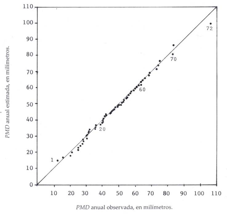
Figure 3 shows the Q-Q graph of the Mexquitic station, whose estimated annual PMD values were obtained with the Wakeby FDP. This fit corresponds to an EEA of 1.45 millimeters, which was the minimum found in the stations of the Potosino Plateau (Table 5).
Results in the middle zone
Concentrate of numerical indexes
The three characteristic values (minimum, medium and maximum) of each index of descriptive ability (HD) obtained with each of the eight contrasting FDPs in the 10 rain-gauge stations of the Middle Zone of the state of San Luis Potosí, Mexico have been integrated in Table 8. Table 8 is similar to Table 5.
Table 8 Characteristic values of the eight descriptive ability (HD) indexes in the 10 series of annual PMD processed of the Middle Zone of the state of San Luis Potosí, México.
| DA Index | contrasted FDP | |||||||
|---|---|---|---|---|---|---|---|---|
| BEK | BEP | LGN | GVE | LOG | PAG | LP3 | WAK | |
| EEA mín | 3.52 | 3.48 | 3.03 | 3.26 | 3.45 | 2.30 | 3.38 | 2.27 |
| EEA med | [8.31] | 8.19 | 6.46 | 6.41 | 6.57 | 7.24 | (6.15) | 7.47 |
| EEA máx | 15.52 | 20.78 | 14.40 | 13.34 | 13.00 | 15.64 | 12.37 | 22.68 |
| EREA mín | 0.043 | 0.043 | 0.045 | 0.048 | 0.044 | 0.034 | 0.045 | 0.0302 |
| EREA med | 0.068 | 0.070 | (0.065) | 0.063 | 0.065 | 0.086 | 0.063 | [0.108] |
| EREA máx | 0.093 | 0.125 | 0.098 | 0.091 | 0.091 | 0.161 | 0.092 | 0.571 |
| EAM mín | 2.361 | 2.382 | 2.112 | 2.312 | 2.424 | 1.768 | 2.225 | 1.653 |
| EAM med | 3.784 | 3.676 | 3.615 | (3.483) | 3.575 | 4.289 | 3.579 | [5.064] |
| EAM máx | 5.247 | 6.292 | 5.437 | 4.864 | 5.638 | 6.611 | 4.870 | 28.199 |
| EAMx mín | 8.8 | 8.4 | 8.7 | 7.7 | 8.3 | 6.1 | 10.6 | 5.8 |
| EAMx med | [47.6] | 46.5 | 32.1 | 31.8 | 32.6 | 35.4 | 29.3 | (26.5) |
| EAMx máx | 105.5 | 150.5 | 94.0 | 88.5 | 87.0 | 100.8 | 78.9 | 79.4 |
| AIC mín | 325.1 | 324.0 | 324.4 | 326.0 | 323.2 | 295.8 | 335.2 | 297.1 |
| AIC med | [423.6] | 417.4 | 396.9 | 396.9 | 400.3 | 406.8 | (394.3) | 401.9 |
| AIC máx | 579.3 | 624.6 | 511.6 | 529.3 | 543.8 | 484.8 | 518.0 | 514.4 |
| COC mín | 0.950 | 0.921 | 0.959 | 0.968 | 0.964 | 0.943 | 0.970 | 0.971 |
| COC med | 0.975 | [0.974] | 0.982 | 0.982 | 0.982 | 0.974 | 0.983 | (0.987) |
| COC máx | 0.991 | 0.991 | 0.992 | 0.991 | 0.991 | 0.995 | 0.991 | 0.992 |
| d 2 mín | 0.964 | 0.944 | 0.971 | 0.975 | 0.976 | 0.965 | 0.979 | 0.800 |
| d 2 med | 0.982 | 0.982 | 0.989 | 0.989 | 0.989 | 0.985 | (0.990) | [0.973] |
| d 2 máx | 0.995 | 0.995 | 0.996 | 0.995 | 0.995 | 0.998 | 0.995 | 0.998 |
| d 1 mín | 0.886 | 0.894 | 0.896 | 0.895 | 0.893 | 0.881 | 0.901 | 0.453 |
| d 1 med | 0.920 | 0.922 | 0.924 | (0.926) | 0.923 | 0.911 | 0.924 | [0.891] |
| d 1 máx | 0.946 | 0.941 | 0.946 | 0.948 | 0.944 | 0.956 | 0.944 | 0.954 |
Concentrate by rain-gauge stations
Table 9 shows for each record of annual PMD processed, which is the best FDP according to each index of descriptive ability. It is observed that the Wakeby distribution is the best option in six stations (Ojo de Agua to San Francisco); in total, it is the best FDP in 42.5% of cases. Based on the results of Table 9, it is concluded that the Wakeby model should always be tested when analyzing annual PMD records of warm-subhumid climates. In the last line of Table 9, the WAK and GVE models can be selected as the second best regional FDP option; the first model was chosen due to its greater number of local occurrences.
Table 9 Best FDP according to each descriptive ability indexes in the 10 series of annual PMD processed of the Middle Zone of the state of San Luis Potosí, Mexico.
| Station | Descriptive ability indexes | Best two FDP* |
|||||||
|---|---|---|---|---|---|---|---|---|---|
| EEA | EREA | EAM | EAMx | AIC | COC | d 2 | d 1 | ||
| Armadillo de los Infante | PAG | LGN | LGN | PAG | PAG | PAG | PAG | WAK | PAG(5), LGN(2) |
| Cárdenas | PAG | LGN | PAG | PAG | PAG | PAG | PAG | PAG | PAG(7), LGN(1) |
| Lagunillas | BEP | LGN | WAK | BEP | BEP | BEP | BEP | WAK | BEP(5), WAK(2) |
| Ojo de Agua | LP3 | WAK | WAK | LP3 | BEP | BEP | LP3 | WAK | WAK(3), LP3(3) |
| Ojo de Agua Seco | WAK | WAK | WAK | BEP | GVE | GVE | BEK | WAK | WAK(4), GVE(2) |
| Paso de San Antonio | WAK | BEP | BEP | WAK | WAK | WAK | WAK | LOG | WAK(5), BEP(2) |
| Rayón | WAK | WAK | WAK | LP3 | LP3 | WAK | WAK | WAK | WAK(6), LP3(2) |
| Río Verde | WAK | WAK | WAK | PAG | PAG | WAK | PAG | WAK | WAK(5), PAG(3) |
| San Francisco | WAK | BEK | WAK | WAK | WAK | WAK | WAK | WAK | WAK(7), BEK(1) |
| San José Alburquerque | LP3 | LP3 | LP3 | WAK | LP3 | LP3 | LP3 | LP3 | LP3(7), WAK(1) |
| Regional | LP3 | LGN | GVE | WAK | LP3 | WAK | LP3 | GVE | LP3(3), WAK(2) |
*Between parenthesis the number of times that occur.
By eliminating the Wakeby distribution from Table 9 and looking for the next best FDP option, the Table 10 is integrated, whose results for the annual PMD records of the Middle Zone place in first and downward order the Generalized Pareto distributions in three stations; Log-Pearson type III, Pareto Beta and Generalized Logistics in two stations. The FDP General of Extreme Values is the best option in one station.
Table 10 Best FDP (excluding Wakeby) according to each descriptive ability index in the 10 series of annual PMD processed in the Middle Zone of the state of San Luis Potosí, Mexico.
| Station | Descriptiva Ability Indexes | Best two FDP* |
|||||||
|---|---|---|---|---|---|---|---|---|---|
| EEA | EREA | EAM | EAMx | AIC | COC | d 2 | d 1 | ||
| Armadillo de los Infante | PAG | LGN | LGN | PAG | PAG | PAG | PAG | LGN | PAG(5), LGN(3) |
| Cárdenas | PAG | LGN | PAG | PAG | PAG | PAG | PAG | PAG | PAG(7), LGN(1) |
| Lagunillas | BEP | LGN | LP3 | BEP | BEP | BEP | BEP | LP3 | BEP(5), LP3(2) |
| Ojo de Agua | LP3 | LOG | BEP | LP3 | BEP | BEP | LP3 | BEP | BEP(4), LP3(3) |
| Ojo de Agua Seco | GVE | BEK | GVE | BEP | GVE | GVE | BEK | GVE | GVE(5), BEK(2) |
| Paso de San Antonio | LOG | BEP | BEP | LOG | BEP | LOG | LOG | LOG | LOG(5), BEP(3) |
| Rayón | LP3 | LOG | BEP | LP3 | LP3 | LOG | LP3 | LOG | LP3(4), LOG(3) |
| Río Verde | PAG | PAG | PAG | PAG | PAG | PAG | PAG | PAG | PAG(8) |
| San Francisco | LOG | BEK | LOG | GVE | LOG | LOG | GVE | LOG | LOG(5), GVE(2) |
| San José Alburquerque | LP3 | LP3 | LP3 | LP3 | LP3 | LP3 | LP3 | LP3 | LP3(8) |
*Between parenthesis the number of times that occur.
Results according to predictive ability
FDPs applied
For each climatological station or annual PMD record, four FDPs were chosen to be contrasted. The first corresponds to the best option in Table 3, that is, it is the most appropriate FDP according to the results of the L-ratio diagram. The following two FDPs to be applied were those obtained as best options according to the eight indexes of descriptive ability, which were concentrated in Table 7 and Table 10. Finally, the Wakeby FDP was applied, due to its great descriptive capacity, which was shown in Table 6 and Table 9; therefore, it is suggested to be applied under precept. In Table 11 and Table 12 of calculated and adopted predictions, the following three stations have been highlighted with bold letters: La Maroma, Río Verde and San José Alburquerque, because in them only three FDPs are contrasted, since in Table 7 and Table 10 report only a better FDP in the eight descriptive ability indexes applied.
Table 11 Predictions of four return periods obtained with the indicated FDPs, in each of the 9 annual PMD series of the Potosino Plateau of the state of San Luis Potosí, Mexico (the predictions adopted are indicated in parenthesis).
| Station Best FDP |
PM (PM /P 50) |
Return periods in years | |||
|---|---|---|---|---|---|
| 50 | 100 | 500 | 1 000 | ||
| Cedral | 315.8 | ||||
| GVE [2] | 2.21 | 143 | 192 | 384 | 520 |
| LP3 (5) | 2.10 | (151) | (206) | (431) | (596) |
| LOG (3) | 2.24 | 141 | 191 | 400 | 555 |
| WAK (4) | 2.32 | 136 | 191 | 443 | 2326 |
| Charcas | 117.0 | ||||
| LGN [3] | 1.10 | 106 | 119 | 147 | 202 |
| LOG (2) | 1.07 | (109) | (126) | (174) | (199) |
| GVE (2) | 1.07 | 109 | 121 | 150 | 162 |
| WAK (6) | 1.07 | 109 | 122 | 150 | 198 |
| La Maroma | 140.1 | ||||
| LOG [1] | 1.30 | 108 | 129 | 197 | 236 |
| BEP (8) | 1.25 | (112) | (136) | (213) | (258) |
| WAK (0) | 1.29 | 109 | 126 | 172 | 279 |
| Los Filtros | 111.0 | ||||
| LP3 [1] | 1.32 | 84 | 93 | 114 | 123 |
| BEK (5) | 1.32 | (84) | (95) | (127) | (143) |
| BEP (2) | 1.35 | 82 | 91 | 117 | 129 |
| WAK (2) | 1.34 | 83 | 93 | 119 | 176 |
| Matehuala | 200.0 | ||||
| LP3 [2] | 1.39 | 144 | 170 | 245 | 285 |
| BEK (5) | 1.29 | (155) | (191) | (309) | (380) |
| LOG (1) | 1.41 | 142 | 171 | 266 | 323 |
| WAK (3) | 1.48 | 135 | 170 | 316 | 1211 |
| Mexquitic | 107.0 | ||||
| LGN [2] | 1.24 | 86 | 91 | 104 | 124 |
| LOG (6) | 1.22 | 88 | 97 | 117 | 127 |
| BEK (1) | 1.32 | 81 | 89 | 111 | 122 |
| WAK (5) | 1.20 | (89) | (98) | (120) | (163) |
| Peñón Blanco | 235.0 | ||||
| LOG [1] | 1.51 | 156 | 216 | 473 | 667 |
| LP3 (5) | 1.39 | (169) | (233) | (490) | (676) |
| GVE (2) | 1.49 | 158 | 217 | 457 | 631 |
| WAK (1) | 1.51 | 156 | 221 | 510 | 2521 |
| Santo Domingo | 270.0 | ||||
| LP3 [1] | 1.61 | 168 | 201 | 293 | 340 |
| BEK (4) | 1.70 | (159) | (198) | (327) | (406) |
| LOG (2) | 1.72 | 157 | 195 | 322 | 400 |
| WAK (2) | 2.03 | 133 | 175 | 400 | 2770 |
| Vanegas | 90.0 | ||||
| LGN [1] | 1.00 | (90) | (102) | (132) | (197) |
| PAG (5) | 1.06 | 85 | 92 | 103 | 107 |
| LP3 (3) | 1.01 | 89 | 101 | 130 | 143 |
| WAK (0) | 1.01 | 89 | 99 | 118 | 146 |
Table 12 Predictions of four return periods obtained with the indicated FDPs, in each of the 10 series of annual PMD of the Middle Zone of the state of San Luis Potosí, Mexico (the predictions adopted are indicated in parenthesis).
| Station Best FDP |
PM (P M /P 50) |
Return periods in years | |||
|---|---|---|---|---|---|
| 50 | 100 | 500 | 1 000 | ||
| Armadillo de los I. | 133.0 | ||||
| LP3 [2] | 0.95 | 140 | 163 | 226 | 258 |
| PAG (5) | 0.99 | 135 | 150 | 180 | 191 |
| LGN (3) | 0.96 | (139) | (162) | (220) | (354) |
| WAK (1) | 0.96 | 138 | 156 | 196 | 267 |
| Cárdenas | 180.5 | ||||
| LP3 [1] | 0.95 | (191) | (231) | (345) | (406) |
| PAG (7) | 0.97 | 186 | 215 | 282 | 311 |
| LGN (1) | 0.95 | 191 | 228 | 330 | 586 |
| WAK (0) | 0.97 | 187 | 216 | 285 | 418 |
| Lagunillas | 210.0 | ||||
| LGN [1] | 1.21 | 173 | 196 | 251 | 368 |
| BEP (5) | 1.16 | (181) | (214) | (317) | (375) |
| LP3 (2) | 1.19 | 176 | 201 | 265 | 295 |
| WAK (2) | 1.22 | 172 | 200 | 289 | 579 |
| Ojo de Agua | 300.2 | ||||
| LOG [1] | 1.31 | (229) | (290) | (510) | (656) |
| BEP (4) | 1.29 | 233 | 293 | 498 | 625 |
| LP3 (3) | 1.27 | 236 | 292 | 474 | 583 |
| WAK (3) | 1.29 | 233 | 298 | 533 | 1623 |
| Ojo de Agua Seco | 172.5 | ||||
| LOG [2] | 1.11 | (155) | (185) | (283) | (341) |
| GVE (5) | 1.12 | 154 | 180 | 252 | 289 |
| BEK (2) | 1.11 | 155 | 185 | 274 | 325 |
| WAK (4) | 1.11 | 155 | 178 | 234 | 356 |
| Paso de S. Antonio | 200.0 | ||||
| GVE [2] | 1.41 | 142 | 161 | 208 | 230 |
| LOG (5) | 1.39 | (144) | (167) | (238) | (277) |
| BEP (3) | 1.42 | 141 | 163 | 228 | 263 |
| WAK (5) | 1.36 | 147 | 172 | 246 | 463 |
| Rayón | 330.0 | ||||
| GVE [2] | 1.63 | 203 | 254 | 427 | 533 |
| LP3 (4) | 1.57 | 210 | 265 | 447 | 558 |
| LOG (3) | 1.63 | (202) | (257) | (461) | (596) |
| WAK (6) | 1.63 | 203 | 267 | 515 | 1834 |
| Río Verde | 126.3 | ||||
| LP3 [3] | 1.00 | (126) | (142) | (184) | (204) |
| PAG (8) | 1.07 | 118 | 125 | 137 | 141 |
| WAK (5) | 1.07 | 118 | 126 | 140 | 153 |
| San Francisco | 135.0 | ||||
| LGN [3] | 1.18 | 114 | 131 | 172 | 260 |
| LOG (5) | 1.15 | 117 | 139 | 208 | 247 |
| GVE (2) | 1.17 | 115 | 134 | 181 | 204 |
| WAK (7) | 1.13 | (119) | (141) | (198) | (342) |
| S. J. Alburquerque | 126.5 | ||||
| GVE [1] | 1.17 | 108 | 121 | 153 | 167 |
| LP3 (8) | 1.13 | (112) | (127) | (167) | (186) |
| WAK (1) | 1.00 | 127 | 137 | 156 | 182 |
When one of the two best FDPs in Table 7 or Table 10 coincided with the first applied distribution, the latter was changed, by its second and/or third option in Table 3. The option that has the first applied FDP was indicated in rectangular parentheses in Table 11 and Table 12 of calculated and selected predictions. For the two best FDPs in Table 7 and Table 10, the number of descriptive ability indexes in which they are the best are indicated in round brackets. The same is indicated for the Wakeby distribution, but such datum comes from Table 6 and Table 9.
Obtained statistics
Table 1 shows that most of the records processed from annual PMD have amplitude of 50 years or more, due to which the quotient between the maximum value of the record (P M ) and the prediction of the 50 year return period (P 50) was calculated. This quotient is indicated in columns 2 of Table 11 and Table 12, and when it is close to the unit it indicates that the record does not have extreme scattered values (outliers) that deviate from the natural trend of the data. On the other hand, when it exceeds 1.50, there is one or more scattered values that is the case of the following four stations: Cedral, Peñón Blanco, Santo Domingo and Rayón.
In the four stations mentioned, the Wakeby distribution, due to its extraordinary flexibility given by its five fitting parameters, leads to very high predictions in the return period of 1000 years; as observed when comparing them with those obtained with the other contrasted FDP. In none of the cases mentioned, the FDP Wakeby was adopted, because its predictions were considered exaggerated, as it did not coincide with those of the other three probabilistic models contrasted in that station. Nguyen et al. (2017) also find that the Wakeby distribution has low predictive ability, by showing great variability in their predictions.
In Table 11 and Table 12 of predictions calculated and adopted in the stations of the Potosino Plateau and the Middle Zone, the descriptive and predictive abilities of each of the contrasted FDP are taken into account implicitly; therefore, the following conclusions are considered globally in the study.
It was obtained that in 12 stations the adopted values come from the two FDPs that were the best option according to the eight indexes of descriptive ability. In five stations the adopted predictions were calculated with the FDP best options according to the L-ratio diagram and only in two stations the predictions calculated with the Wakeby distribution were adopted.
As already indicated, exclusively in three stations; La Maroma, Río Verde and San José Alburquerque, a total concordance was obtained in the eight indexes of descriptive ability, for the FDP Beta-P, Generalized Pareto and Log-Pearson type III, respectively. These stations have been highlighted in bold in Table 11 and Table 12.
By geographic areas, in the Potosino Plateau of nine processed records, the FDP Beta-κ was the model adopted in three stations and the Log-Pearson type III distribution in two stations. In the Middle Zone of 10 processed records, the FDP Generalized Logistics with four stations had a preponderance of adoption and was followed by the LP3 distribution with three stations.
Conclusions
The Wakeby distribution, fitted with the L-moment method is a model of excellent descriptive ability and therefore, it is suggested to be applied under precept in the probabilistic analyzes of annual PMD records of the arid and semi-arid climates of the Potosino Plateau (AP) and of the warm-subhumid climate of the Middle Zone (ZM) of the state of San Luis Potosí, Mexico.
The Beta-κ and Beta-P distributions, fitted with the maximum likelihood method, are models not applied in Mexico that are suggested to be tested, since for four annual PMD records of the AP (Table 7) and two of the ZM (Table 10), lead to the best descriptive ability indexes.
Regarding the distributions that are applied under precept in the USA and England, it was obtained (Table 7 and Table 10): (1) the FDP Log-Pearson type III that proved to be the best option in two stations of the AP and ZM; (2) the FDP General of Extreme Values only in one station of the ZM was a better option; (3) the FDP Generalized Logistics was the best option in two stations of the AP and ZM. (4) In the AP the Generalized Logistics stands out as the second best option and in the ZM the Log-Normal and Log-Pearson models type III.
Regarding the FDP Generalized Pareto, which is commonly applied together with the LOG and GVE models; it was a better option in one station of the AP and three in the ZM. These results confirm the systematic application or under precept of LP3, GVE, LOG and PAG distributions in annual PMD series of arid, semi-arid and warm-sub-humid climates.
Regarding the calculated predictions (Table 11 and Table 12) in the return periods of 50, 100, 500 and 1000 years, they generally show similar values and this generates confidence in the adopted values. Dispersion was exclusively found in the predictions of the FDP Wakeby, in the stations or records of annual PMD with extreme scattered value (outlier), in case of the stations: Cedral, Peñón Blanco, Santo Domingo and Rayón.
Regarding the adopted predictions (Table 11 and Table 12) it is concluded that the search procedures for the best FDP to be applied to the annual PMD records, based on the L-ratio diagrams and on the eight descriptive ability indexes, are adequate and lead to a good approximation, since there was not difficulty to select the adopted predictions.
Referencias
Asquith, W. H. (2011). L-moments. Chapter 6. In: Distributional analysis with L-moments statistics using the R environment for statistical computing (pp. 87-122). Lubbock, USA: United States Geological Services. [ Links ]
Benson, M. A. (1962). Plotting positions and economics of engineering planning. Journal of Hydraulics Division, 88(6), 57-71. [ Links ]
Bobée, B., & Ashkar, F. (1991). The Gamma Family and derived distributions applied in Hydrology. Littleton, USA: Water Resources Publications. [ Links ]
Campos-Aranda, D. F. (2002). Contraste de seis métodos de ajuste de la distribución Log-Pearson tipo III en 31 registros históricos de eventos máximos anuales. Ingeniería Hidráulica en México, 17(2), 77-97. [ Links ]
Campos-Aranda, D. F. (2015). Ajuste de las distribuciones GVE, LOG y PAG con momentos L depurados (1,0). Tecnología y ciencias del agua, 6(4), 153-167. [ Links ]
Campos-Aranda, D. F. (2016). Ajuste de las distribuciones GVE, LOG y PAG con momentos L de orden mayor. Ingeniería, Investigación y Tecnología, 17(1), 131-142. [ Links ]
Campos-Aranda, D. F. (2018). Estimación estadística actualizada de la PMP en el estado de San Luis Potosí, México. Tecnología y ciencias del agua , 9(6), 32-70. [ Links ]
Chai, T., & Draxler, R. R. (2014). Root mean square error (RMSE) or mean absolute error (MAE)? Arguments against avoiding RMSE in the literature. Geoscientific Model Development, 7, 1247-1250. [ Links ]
Coles, S. (2001). Model diagnostics. Theme 2.6.7. In: An introduction to statistical modeling of extreme values (pp. 36-44). London, England: Springer-Verlag. [ Links ]
Cunnane, C. (1978). Unbiased plotting positions. A review. Journal of Hydrology, 37(3-4), 205-222. [ Links ]
Haktanir, T. (1991). Statistical modeling of annual maximum flows in Turkish rivers. Hydrological Sciences Journal, 36(4), 367-389. [ Links ]
Haktanir, T. (1992). Comparison of various flood frequency distributions using annual flood peaks of rivers in Anatolia. Journal of Hydrology, 136(1-4), 1-31. [ Links ]
Hosking, J. R. M., & Wallis, J. R. (1997). Regional frequency analysis. An approach based on L-moments. Cambridge, England: Cambridge University Press. [ Links ]
Houghton, J. C. (1978). Birth of a parent: The Wakeby distribution for modeling flood flows. Water Resources Research, 14(6), 1105-1109. [ Links ]
Johnson, F., & Sharma, A. (2017). Design rainfall. Chapter 125. In: Singh, V. P. (ed.). Handbook of applied hydrology, 2nd ed. (pp. 125.1-125.13). New York, USA: McGraw-Hill Education. [ Links ]
Kite, G. W. (1977). Chapter 12: Comparison of frequency distributions. In: Frequency and risk analyses in hydrology (pp. 156-168). Fort Collins, USA: Water Resources Publications. [ Links ]
Legates, D. R., & McCabe, G. J. (1999). Evaluating the use of “goodness-of-fit” measures in hydrologic and hydroclimatic model validation. Water Resources Research , 35(1), 233-241. [ Links ]
Machiwal, D., & Jha, M. K. (2008). Comparative evaluation of statistical tests for time series analysis: Applications to hydrological time series. Hydrological Sciences Journal, 53(2), 353-366. [ Links ]
Mujumdar, P. P., & Nagesh-Kumar, D. N. (2012). Floods in a changing climate. Hydrologic modeling. Cambridge, United Kingdom: International Hydrology Series (UNESCO) and Cambridge University Press. [ Links ]
Meylan, P., Favre, A. C., & Musy, A. (2012). Predictive hydrology. A frequency analysis approach. Boca Raton, USA: CRC Press. [ Links ]
Mielke, P. W., & Johnson, E. S. (1974). Some generalized Beta distributions of the second kind having desirable application features in Hydrology and Meteorology. Water Resources Research , 10(2), 223-226. [ Links ]
Nguyen, T. H., El Outayek, S., Lim, S. H., & Nguyen, T. V. T. (2017). A systematic approach to selecting the best probability models for annual maximum rainfalls - A case study using data in Ontario (Canada). Journal of Hydrology , 553, 49-58. [ Links ]
Pandey, G. R., & Nguyen, V. T. V. (1999). A comparative study of regression based methods in regional flood frequency analysis. Journal of Hydrology , 225(1-2), 92-101. [ Links ]
Peel, M. C., Wang, Q. J., Vogel, R., & McMahon, T. A. (2001). The utility of L-moment ratio diagrams for selecting a regional probability distribution. Hydrological Sciences Journal, 46(1), 147-155. [ Links ]
Rao, A. R., & Hamed, K. H. (2000). Probability weighted moments and L-moments. Chapter 3 (pp. 53-72). In: Flood frequency analysis. Boca Raton, USA: CRC Press . [ Links ]
Stedinger, J. R. (2017). Flood frequency analysis. Chapter 76. In: Singh, V. P. (ed.). Handbook of applied hydrology, 2nd ed. (pp. 76.1-76.8). New York, USA: McGraw-Hill Education . [ Links ]
Teegavarapu, R. S. V. (2012). Floods in a changing climate. Extreme precipitation. Cambridge, United Kingdom: International Hydrology Series (UNESCO) and Cambridge University Press. [ Links ]
Willmott, C. J., & Matsuura, K. (2005). Advantages of the mean absolute error (MAE) over the root mean square error (RMSE) in assessing average model performance. Climate Research, 30(1), 79-82. [ Links ]
Wilks, D. S. (1993). Comparison of three-parameter probability distributions for representing annual extreme and partial duration precipitation series. Water Resources Research , 29(10), 3543-3549. [ Links ]
Wilks, D. S. (2011). Statistical Methods in the Atmospheric Sciences. Theme 4.5: Qualitative assessments of the goodness fit, pp. 112-116. San Diego, USA: Academic Press (Elsevier). Third edition. 676 p. [ Links ]
WMO, World Meteorological Organization. (1971). Climatic change. Annexed III (pp. 58-71) (Technical Note No. 79). Geneva, Switzerland: Secretariat of the World Meteorological Organization. [ Links ]
WRC, Water Resources Council. (1977). Guidelines for determining flood flow frequency. Bulletin # 17A of the Hydrology Committee (Revised edition). Washington, DC, USA: Water Resources Council. [ Links ]
Yue, S., & Hashino, M. (2007). Probability distribution of annual, seasonal and monthly precipitation in Japan. Hydrological Sciences Journal, 52(5), 863-877. [ Links ]
Zalina, M. D., Desa, M. N. M., Nguyen, V. T. V., & Kassim, A. H. M. (2002). Selecting a probability distribution for extreme rainfall series in Malaysia. Water Science and Technology Journal, 45(3), 63-68. [ Links ]
Received: November 16, 2017; Accepted: November 22, 2018
 Este es un artículo publicado en acceso abierto bajo una licencia Creative Commons
