


Services on Demand
Journal
Article
 text in
  English (pdf)
 Article in xml format
 Article references
 Send this article by e-mail
Indicators
-
 Cited by SciELO
 -
 Access statistics
Related links
-
 Similars in
SciELO
Similars in
SciELO
Share

 Permalink
Tecnología y ciencias del agua
On-line version ISSN 2007-2422
Tecnol. cienc. agua vol.9 n.4 Jiutepec Jul./Aug. 2018 Epub Nov 24, 2020
https://doi.org/10.24850/j-tyca-2018-04-09
Articles
Comparison of physical models and artificial intelligence for prediction of flood levels
1Universidad de La Sabana, Chía, Cundinamarca, Colombia, mauricioao@unisabana.edu.co
2Universidad de La Sabana, Chía, Cundinamarca, Colombia, william.moscoso@unisabana.edu.co; Universidad Central, Chía, Cundinamarca, Colombia, wmoscosob@ucentral.edu.co
3Universidad de La Sabana, Chía, Cundinamarca, Colombia, luis.paipa@unisabana.edu.co
4Universidad de La Sabana, Chía, Cundinamarca, Colombia, catalinamesc@unisabana.edu.co
Hydrology has used traditional methods for flood level forecasting. However, this type of forecast can lead to accuracy issues, caused by the nonlinear behavior of floods and limitations by not including all variables, such as water flow, level and precipitation. Consequently, some scientists began to use unconventional methods based on artificial intelligence models, to forecast floods more precisely and rigorously. This paper compares the HEC-RAS one-dimensional flow transit model with an artificial intelligence model based on Artificial Neural Networks, developed in MatLab to predict floods. The results were analyzed using six statistical indicators: mean absolute error (MAE), mean squared error (MSE), mean absolute percentage error (MAPE), square root of the MSE, Pearson correlation coefficient (CC), and concordance correlation coefficient (ρc). In addition, the efficiency coefficient was calculated, and used in a virtual tool called Hydrotest. The analysis shows that forecast models that use neural networks have accurate results, given their closeness to the real data: MAPE between 11.95 and 12.51, CC between 0.90 and 0.92, ρc between 0.84 and 0.87, and a coefficient of efficiency larger than 0.8. The study was conducted on a section of the upper Bogotá River, in Colombia, between the Florence Bridge and Tocancipá hydrological stations. Flow data was taken from the Regional Autonomous Corporation of Cundinamarca (CAR), from September 2009 to October 2013.
Keywords Artificial neural networks; HEC-RAS; physical model; intelligent model; flood forecasting
La hidrología ha utilizado métodos tradicionales para pronosticar niveles de inundación. Sin embargo, éstos pueden generar problemas de precisión, causados por el comportamiento no lineal de las inundaciones y las limitaciones al no incluir todas las variables, como flujo, y nivel de agua y precipitación. En consecuencia, algunos científicos comenzaron a utilizar métodos no convencionales basados en modelos de inteligencia artificial, pronosticando las inundaciones de manera más precisa y rigurosa. Este artículo presenta una comparación de un modelo de tránsito de flujo unidimensional desarrollado en HEC-RAS y un modelo de inteligencia artificial, basado en redes neuronales artificiales, desarrollado en MatLab, para predecir inundaciones. El análisis de los resultados se llevó a cabo utilizando seis indicadores estadísticos: error absoluto medio (MAE, por su nombre en inglés); error cuadrático medio (MSE); error medio porcentual absoluto (MAPE, por su nombre en inglés); raíz cuadrada de la MSE; coeficiente de correlación de Pearson (CC, por su nombre en inglés), y coeficiente de correlación de concordancia (ρc, por su nombre en inglés). Además, el coeficiente de eficiencia se calculó empleando una herramienta virtual llamada Hydrotest. A partir del análisis se observó en los modelos de pronóstico que el uso de redes neuronales tiene resultados precisos, dada su cercanía con los datos reales: MAPE, entre 11.95 y 12.51; CC, entre 0.90 y 0.92; ρc, entre 0.84 y 0.87, y finalmente un CE más grande que 0.8. El estudio se realizó en una sección de las partes altas del río Bogotá, en Colombia, entre las estaciones hidrológicas de puente Florencia y Tocancipá. Los datos de flujo fueron tomados por la Corporación Autónoma Regional de Cundinamarca (CAR) de septiembre de 2009 a octubre de 2013.
Palabras clave redes neuronales; HEC-RAS; modelo físico; modelo inteligente; pronóstico de inundaciones
Introduction
Flooding is a natural phenomenon which occurs when rainfall occurs frequently or is so strong that the soil’s absorption capacity is exceeded, causing water to change course and extend into adjacent areas (SDAB, 2009). The consequences become more drastic when occurring in populated urban areas, since this involves not only environmental but also social and economic damage. Government entities must then divert large amounts of resources originally allocated for other sectors (i.e. education and health) to recover flooded spaces and infrastructure (CAR, 2016). World Bank data (Banco Mundial Colombia, 2012) has shown that flooding causes 43% of destroyed homes and about 10% of the loss of human lives.
Two events having great climatic variability, which represent the greatest threat in Colombia, are the phenomena called “El Niño” and “La Niña.” The former is characterised by droughts and a lack of water, thereby producing forest fires, whilst “La Niña” involves greater soil saturation, which causes events such as landslides and flash floods, especially in Colombia’s Andean, Caribbean and Pacific regions. A state of economic, social and ecological emergency was declared throughout Colombia in January 2011 due to the devastating effects of flooding. The Corporación Autónoma Regional (CAR), the entity that manages the River Bogota Basin, argues that probabilistic models are needed for estimating climatic variability and identifying any increase in the volume of rivers, since they can be used to generate natural disaster alerts and provide useful information for decisions regarding emergency prevention (CAR, 2016).
Hydrology has traditionally used one-dimensional methods for forecasting flows, with which flooding is determined by linear regression (Pandey & Nguyen, 1999). This method measures the relationship between the dependent and independent variables (Weisberg, 2005). Drawbacks from this approach include problems and limitations in terms of prediction, not just due to climate change affecting the earth (Huffman, 2001), or difficulties regarding calibration and the robust optimisation tools needed (Kia et al., 2011), but also because these types of phenomena are not linear, thereby making the use of this type of predictive model unsuitable (Dawson, Abrahart, Shamseldin, & Wilby, 2006; Aqil, Kita, Yano, & Nishiyama, 2007). As stated above, while traditional methods have proved extremely helpful in predicting floods, researchers have now taken to studying more effective models having greater accuracy in forecasting.
Another way of forecasting floods is to use physical models based on hydraulic principles. This makes it possible to explain river flow patterns through physical laws linked to differential equations. Saint-Venant equations have been studied; they have been useful in representing water flow models. However, it has been shown that they sometimes produce unstable solutions due to a great accumulation of errors when the flow depth increases rapidly, thereby requiring more complex mathematics and more precise modelling (Amarís, Guerrero, & Sanchez, 2015).
Another difficulty related to physical models is the amount of information they require in terms of hydro-meteorological variables (flow, water level, rainfall), in addition to the geological and topographic aspects of a particular channel (i.e. bathymetry (underwater terrain depths and shapes), and soil types, flow curves and runoff parameters (Merwade, Cook, & Coonrod, 2008; Kia et al., 2011). The forgoing limits the use of this type of model, since certain basins have not been characterised in terms of their storage capacity, water catchment, and the likely flood zones along the rivers in question (Werner, Gallagher, & Weeks, 2006; Park, Joo, & Kim, 2012; Callow & Boggs, 2013).
The physical model analysed in this research is a transit time model for flow, which predicts changes in the magnitude, velocity and shape of a flow wave as a function of time (hydrograph) at one or more points along a river or canal (Chow, Maidment, & Mays, 1994). This one-dimensional modelling involved using the Hydrologic Engineering Center’s (CEIWR-HEC) River Analysis System (HEC-RAS) software, created by the US Army Corps of Engineers (US Army Corps Engineers & Hydrologic Engineering Center, 2016). This has been used in work involving hydraulic simulation (Manfreda et al., 2014; Guida, Swanson, Remo & Kiss, 2015; Dimitriadis et al., 2016).
HEC-RAS software has also been used for analysing the risk of flooding with 3D, 2D and 1D hydraulic simulation systems (Zazo, Molina, & Rodríguez-González, 2015).
Studies of prediction models have been developed for future events, integrating artificial intelligence system techniques, which have a flexible mathematical structure capable of modelling complex nonlinear relationships between input and output data characteristics; this is difficult to describe using physical equations (Seckin, Cobaner, Yurtal, & Haktanir, 2013). Artificial neural networks (ANN) represent one of the most used techniques in the field of artificial intelligence for flood forecasting worldwide. They simulate the brain’s functioning for resolving problems through mathematical models inspired by neurological processes (Kalteh, 2013; Wang, Chau, Cheng, & Qiu, 2009). Another technique involves linking ANN with an adaptive network-based fuzzy inference system (ANFIS), which is used for building forecast models (Aqil et al., 2007). Table 1 gives some cases of ANN being used as a prediction system.
Table 1 Examples of using artificial neural network (ANN) models.
| Author | Application |
|---|---|
| Kalteh (2013) | Developing prediction models using artificial intelligence techniques |
| Nastos, Paliatsos, Koukouletsos, Larissi, & Moustris (2014) | Predicting daily maximum rainfall using multiple linear regression models and artificial neural networks |
| Tisseuil, Vrac, Lek & Wade (2010) | Evaluating statistical (downscaling) models, such as ANN neural networks, for predicting climate change considering hydrological resources |
| Yilmaz, Imteaz, & Jenkins (2011) | Predicting snow-related catchment flows, evaluating runoff data based on meteorological history |
| Taormina, Chau, & Sivakumar (2015) | Predicting a river’s flow with base flow separation and binary-coded swarm optimisation |
| Deo & Şahin (2016) | Making an extreme learning machine (ELM) for simulating monthly mean flow levels in eastern Queensland, Australia, comparing the performance of flow prediction models with that of artificial neural networks |
| Appelhans, Mwangomo, Hardy, Hemp, & Nauss (2015) | Predicting temperature patterns on mount Kilimanjaro, using machine learning approaches involving 14 learning algorithms |
| Deo & Şahin (2015) | Predicting monthly standardised precipitation (SPI) and standardised precipitation evapotranspiration index (SPEI) |
Artificial intelligence techniques are currently being used as a reference for research dealing with predicting future events, because they emulate a particular phenomenon’s non-linear behaviour, thereby resulting in a more successful forecast (Zou, Xia, Yang, & Wang, 2007). Artificial intelligence techniques help in making appropriate decisions regarding water use, particularly in the field of hydrology.
This article compares a physical model to an intelligent model for predicting flood levels along a stretch of the River Bogota basin (Colombia) between the Puente Florencia (satellite) and Tocancipá hydrological stations.
Materials and methods
The HEC-RAS hydrological model
This tool enables hydraulic modelling of a water’s permanent and temporary flow patterns in artificial canals and natural channels, including rivers (US Army Corps Engineers & Hydrologic Engineering Center, 2006). This software’s hydraulic simulation is based on deterministic differential equations that enable the prediction of water level dynamics that occur during events with high rainfall that cause flooding. Flood levels are defined by cross-sectional profiles. The dynamics of the water and channel behaviour are simulated, including: cross-sections having any type of geometry along a channel, different depths of water and variable flow along a channel in sub-critical or super-critical flow conditions, having hydraulic effects due to natural or artificial transverse obstacles in the channel (Sarhadi, Soltani, & Modarres, 2012; Mohammadi, Nazariha, & Mehrdadi, 2014).
HEC-RAS software (for the simulation model used in this research) uses a continuity equation (US Army Corps Engineers & Hydrologic Engineering Center, 2006) that describes the conservation of mass for a one-dimensional system, as well as calculates storage terms:
where x = distance along the channel, t = time, Q = flow, A = cross- section area, S = storage and q 1 = lateral input per unit of distance.
The following calibration parameters were used in the modelling:
Hydrographs: graphs enabling the flow rate or flow to be observed at a given point on the current (Chow et al., 1994).
Flow curves or calibration curves: graphical representations of the relationship between the water level and its respective flow (Salazar & Chaparron, 1990).
Cross-sections: these define a river’s shape and geometric characteristics and must be topographically connected so that they define the longitudinal profile.
where K = cross-section, n = Manning coefficient of roughness for the section, A = the section’s flow area and R = the section’s hydraulic ratio (area/wetted perimeter).
Manning’s roughness coefficient: also called the roughness coefficient, which enables a channel’s runoff resistance to be estimated (Ruberto, Carreras, & Depettris, 2003). When there are several Manning coefficients (nc) for a channel’s roughness. The main channel is divided into N parts, each having a wetted perimeter Pi and a roughness coefficient n i :
where n c = composite roughness coefficient; P = main channel wetted perimeter; P i = wetted perimeter of section I, and n i = roughness coefficient per section.
Research using this software usually evaluates how well a hydraulic model predicts floods, in order to identify vulnerable areas, critical infrastructure and the affected land use value (Sarhadi et al., 2012; Zazo et al., 2015). Studies have demonstrated that HEC-RAS modelling enables different scenarios to be evaluated for forecasting areas of flooding (Guida et al., 2015). This software is also used for optimising the geometric visualization of areas prone to flooding, which can be subsequently visualised using a geographic information system (GIS) (Sarhadi et al., 2012). Mohammadi et al. (2014) simulated flooding and hydraulic conditions in flood areas for different return periods (recurrence intervals) using HEC-RAS, HEC-GEORAS and GIS models in a case study, presenting their results as risk analysis and flood damage.
Artificial neural network (ANN) model
A standard ANN structure (Figure 1) consists of a set of neurons organised into a hierarchy of layers (input, hidden and output) constituting an autonomous functional system (Chen, Chen, Chou, & Yang, 2010). The following elements can be identified with this type of intelligent system: input and output variables and synaptic weights (the intensity of interaction between neurons and propagation, activation and output functions) (Komatsu et al., 2014). The amount of layers and neurons represents one of the most important parameters in ANN since that determines a system’s efficiency.

One of ANNs’ advantages is that they are useful tools for modelling when the ratio of entry data to output data is unknown (which is why this type of model is called a black box) (Chau, Wu, & Li, 2005; Wang, Wang, Lei, Jiang, & Song, 2011), enabling complex systems to be modelled based on their mathematical composition (i.e. hydrological processes) (Dawson et al., 2006). Another benefit is that ANNs can produce output from a specific combination of inputs, and their response capability concerning managing non-linear data (Santillán, Fraile-Ardanuy, & Toledo, 2014; Cervantes-Osornio, Arteaga-Ramírez, Vázquez-Peña, Ojeda-Bustamante, & Quevedo-Nolasco, 2013).
Available data
The Bogota River basin is located in Colombia’s Cundinamarca department. It has a 5 891 km2 surface area, representing around 32% of the department’s total surface area. The Bogota River is the basin’s main river; it runs for a total of 308 kilometres from an altitude of 3 300 metres above sea level (masl) in the municipality of Villapinzón to its outlet into the Magdalena River at 280 masl in the municipality of Girardot (CAR, 2006).
The Bogota River is divided into 3 sub-basins: upper, middle and lower. The stretch being studied was in the upper basin (Figure 2) between the Puente Florencia hydrological station in the municipality of Gachancipá (upstream) and the Tocancipá station in the municipality of Tocancipá (downstream). This stretch is characterised by having hourly flow frequency records available and stability regarding such records (i.e. there is no reservoir or other large water body nearby that significantly alters the basin’s hydrological pattern).
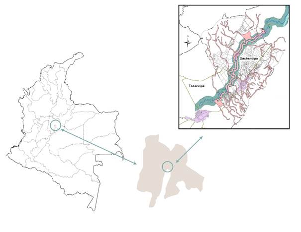
Figure 2 The study segment (authors, with cartography supplied by the CAR and IGAC). Regional Autonomous Corporation (Corporación Autónoma Regional - CAR), Agustín Codazzi Geographical Institute (Instituto Geográfico Agustín Codazzi, IGAC).
Twelve small sub-basins were identified as contributing flows to the section being studied, which added together, considerably increase the river’s level during periods of heavy rainfall. The rational formula method (estimating peak runoff rate at a specific location as a function of drainage network area, runoff coefficient, and mean rainfall intensity) was used for calculating each sub-basin’s contribution to flow, using the water level curves corresponding to each sub-basin and flow order (Horton, 1945).
Physical model produced using HEC-RAS software
The physical model implemented in HEC-RAS required establishing the calibration parameters, with which the flows were simulated at the output of the model. The parameters used for simulating the model’s output flows were as follows: hydrographs from the Puente Florencia and Tocancipá stations, flow curves or calibration curves, cross- sections and Manning roughness coefficient.
Data from April, May, October and November 2011 and 2013 were taken for simulating the (branch-network) flow model as flooding occurred during these dates due to heavy rainfall.
Concerning the flow curves, upstream at the Puente Florencia station, a maximum of roughly 60 m3/s can occur at a 5-meter water level height. And downstream at the Tocancipá hydrological station a maximum of roughly 50 m3/s at a 5-meter water level height can occur.
Regarding the model’s cross-sections, bathymetry was used for taking measurements at points in the field; 151 sections from the study segment were used, with distances varying from 100 to 800 meters in length, depending on the shape of the channel (i.e. measurements were made at shorter distances in areas having very tight curves).
Manning’s roughness coefficient was calibrated based on constant friction with the surface and the surface with the least friction on the sides of the channel.
Calibrating the one-dimensional hydraulic model simulated in HEC-RAS began by identifying a simple hydrograph showing a wave without distortions, during a period of time in which average flows occurred in the study segment, using Manning coefficients ranging from 0.021 - 0.04 for all cross-sections (Santos, Cubillos, & Vargas, 2008; Cook & Merwade, 2009). With the aforementioned characteristics in mind, the period from the 12th to the 23rd of July 2010 was chosen, based on which the Puente Florencia station’s hydrographs and the calculated flows from the 12 sub-basins were entered in the (HEC-RAS) database.
Three scenarios (January, April to June, and October) were simulated for 2011 and 2013 after calibrating Manning coefficients. The parameter concerning the last cross-section (i.e. the Tocancipá station or the model’s output) was configured with a normal 0.0001 depth value, this being suitable for situations where flow approaches uniform rate (US Army Corps Engineers & Hydrologic Engineering Center, 2006).
Artificial neural network (ANN) model
MATLAB Neural Network Toolbox (2013) software was used for ANN simulation, with flow data from the Puente Florencia station and from the 12 sub-basins along the study segment as input, and flows at the Tocancipá station as the model’s output.
The data was normalised between -1 to 1 (Matworks, 2013), giving an input entry for the model using the Puente Florencia station’s flows and those from the 12 sub-basins along the study segment. The model’s output was a vector from the ANN flow data calculated for the Tocancipá station.
Accurately training the ANN and its forecasts involved dividing the data into two parts. Data from September 2009 to December 2012, including February, March, July, August and September 2013, were used for training (70%), whereas data (the remaining 30%) from January, April, May, June and October 2011 and 2013 were used for forecasting.
MATLAB’S Neural Network Toolbox was configured using backpropagation training (Kia et al., 2011; Chen et al., 2010). The Levenberg-Marquardt backpropagation algorithm was used for the learning function (trainlm), this being the fastest algorithm for this type of training with large networks. It adjustment function performs better for recognising a target system’s patterns (Matworks, 2013). The following parameters were configured in the Toolbox in order to run the model: a maximum 2 000 iterations (repetitions), 1e-05 minimum gradient and a maximum of 6 validation reviews for evaluating the model’s quality.
A multilayer structure was used for training every scenario (Kia et al., 2011; Siou, Johannet, Borrell, & Pistre, 2011), modifying the amount of layers (2 to 20) and neurons (2 to 50). Altogether, 168 scenarios were trained as input layers and divided into hidden layers according to their propagation function: 85 had a sigmoid-sigmoid configuration and 83 a sigmoid-linear configuration. A forecast was simulated for every scenario and a MATLAB programme used the results for ascertaining the model’s efficiency.
The models’ statistical evaluation criteria
After the simulations had been made, resulting in the Tocancipá station’s output hydrographs for each period, these were compared to real data for the same periods of time. The following six statistical indexes were used for data analysis, which have been used in most articles consulted and as a method to evaluate the performance of simulation models) (Dawson, Abrahart, & See, 2007): mean absolute error (MAE) (Singhal & Swarup, 2011), mean squared error (MSE) (Gomes & Ludermir, 2013), mean absolute percentage error (MAPE) (Lewis, 1982), root-mean-squared error (RMSE) (Singhal & Swarup, 2011), Pearson’s correlation coefficient (CC) (Lin, Hedayat, Bikas, & Yang, 2002), and concordance correlation coefficient (ρc) (Lin, 2011).
The results of this research were also compared to HydroTest Statistical Assessment of Hydrological Forecasts, which evaluated 20 statistical measures reported by hydrological modelling studies (Dawson et al., 2007). Four HydroTest metrics were used for evaluating real data and modelled data (HEC-RAS, ANN sig-lin and ANN sig-sig) (i.e. 30% of the data selected for validation).
Results
Table 2 shows the results of the HEC-RAS simulated model, with six statistics. As can be seen, a ρc of 0.86 was obtained, indicating that the model had a high ratio of real to simulated data, in terms of accuracy and precision. The correlation coefficient (CC) indicated less than 10% error regarding simulated data ratio (i.e. the error was low). MAE, MSE and RMSE values were also low, indicating little differences regarding real data; this shows a good forecast since the MAPE value was 11%-20% (Lewis, 1982).
Table 2 Statistical comparison of real data to HEC-RASsimulated data.
| Statistical method | ρc | CC | MAE | MAPE | MSE | RMSE |
|---|---|---|---|---|---|---|
| Value | 0.8601 | 0.9077 | 2.2311 | 11.9535 | 15.7725 | 3.9715 |
The three scenarios having the highest ANN MAE, MAPE, MSE, RMSE, CC and ρc values were then chosen for each network configuration. Table 3 shows the best three scenarios for each configuration obtained with the ANN model.
Table 3 The best ANN scenarios.
| Function | Acceptance | Largest coefficient | Largest coefficient | Least error | < 20 % MAPE | Least error | Least error |
|---|---|---|---|---|---|---|---|
| Criteria | ρc | CC | MAE | MAPE | MSE | RMSE | |
| Sigmoid-sigmoid | Scenario 3 | 0.8639 | 0.9032 | 2.0652 | 13.4254 | 12.2868 | 3.5052 |
| Scenario 4 | 0.8667 | 0.9035 | 2.0604 | 13.4697 | 12.2299 | 3.4971 | |
| Scenario 9 | 0.8770 | 0.9215 | 1.9007 | 11.9590 | 10.1782 | 3.1903 | |
| Sigmoid-linear | Scenario 2 | 0.8729 | 0.9136 | 1.9462 | 12.5194 | 10.9753 | 3.3129 |
| Scenario 3 | 0.8593 | 0.9108 | 2.0435 | 12.6997 | 11.6512 | 3.4134 | |
| Scenario 6 | 0.8731 | 0.9104 | 1.9834 | 13.0086 | 11.3318 | 3.3663 |
Discussion
After analysing all the statistical criteria regarding the best scenarios, it was determined that scenario 9 (consisting of 20 layers having 25 neurons in each layer) had the best sigmoid-sigmoid propagation function, given that its results met the greatest amount of statistical criteria: least MAE (1.90), least MAPE (11.9%), least MSE (10.2), least RMSE (3.2), highest CC (0.92) and highest ρc (0.88). Taking the MAPE result as a reference, the forecast was found to be good, ranging from 11% to 20% (Lewis, 1982), and the CC indicated that the model had 92% forecast accuracy in terms of the real data to simulated data ratio.
Regarding the sigmoid-linear propagation function, scenario 2 (consisting of 2 layers having 50 neurons) was chosen as the best forecast because it had the greatest amount of favourable results regarding the statistical criteria evaluated: least MAE (1.94), least MAPE (12.5%), least MSE (10.97), least RMSE (3.1) and highest CC (0.914) 0.914.
Regarding the amounts of neurons, both configurations resulted in the best forecast, having a considerable amount of them in each layer.
Comparing the physical model to artificial intelligence models
A literature search revealed investigations that compared mathematical models (such as linear regression or multiple regression) to intelligent artificial systems, concluding that intelligent systems had a higher real data to simulated data ratio (Aqil et al., 2007; Firat & Güngör, 2007; Kisi, Shiri, & Nikoofar, 2012; Karimi, Kisi, Shiri, & Makarynskyy, 2013), thereby providing a better forecast than mathematical models. However, the search did not find evidence of hydraulics or traditional hydrology studies that made a comparison with a physical model, which is why this comparison was made. It was found that traditional statistical criteria (CC, MAE, MAPE, RSME) were used in such research but none involved analysis using the concordance correlation coefficient (ρc), which indicates the relationship between a model’s precision and its accuracy (Firat & Gürgör, 2007).
The results were used for comparing the HEC-RAS simulated physical model to the best two ANN MATLAB models. Table 4 gives the results for the three best models. The data suggests that the models had very similar forecasts; the sigmoid-sigmoid ANN, the sigmoid-linear ANN and HEC-RAS models are shown in order of effectiveness.
Table 4 Results regarding the best HEC-RAS and ANN models.
| Acceptance | Highest coefficient | Highest coefficient | Least error | <20% MAPE | Least error | Least error |
|---|---|---|---|---|---|---|
| Model | ρc | CC | MAE | MAPE | MSE | RMSE |
| HEC-RAS | 0.8601 | 0.9077 | 2.2311 | 11.9535 | 15.7725 | 3.9715 |
| Sig-sig ANN | 0.877 | 0.9215 | 1.9007 | 11.959 | 10.1782 | 3.1903 |
| Sig-lin ANN | 0.8729 | 0.9136 | 1.9462 | 12.5194 | 10.9753 | 3.3129 |
Figure 3 compares the best three models used in the research (HEC-RAS, sigmoid-sigmoid ANN and sigmoid-linear ANN) and the real data to simulated data ratio using a reference line. It should be noted that 30% of the total flow data was used to validate the models in this simulation.

For the Tocancipá station, real output flow data compared to simulated data was found above and below the reference line in this figure. If data were above it then the flow forecast would be overestimated and if the data were below the flow forecast it would have been underestimated.
It can be seen that the HEC-RAS model shown in Figure 3a underestimated output flow, since most of the data were below the reference line, meaning that it could not predict flooding levels. Whereas data predicted by the ANN models (sig-sig Figure 3b and sig-lin 3c) had a more homogeneous dispersion, with data above and below the reference line, indicating that it would have a greater possibility of predicting flooding levels corresponding to high flows at the model’s output.
Table 4 shows that the sigmoid-sigmoid configuration resulted in the best ANN model. Hydrographs were then drawn after selecting the best intelligent model in order to compare real flow data to simulated flow data for a period of heavy rainfall, as in April 2011.
As can be seen, the simulated values in the HEC-RAS model’s hydrograph shown in Figure 4a were found to be lower than the real ones, meaning that the physical model did not properly predict the real flows that occurred during that period. The model would thus not be reliable for predicting future flooding events.
Figure 4b shows that the selected ANN model better predicted real flows during the same period as that shown in Figure 4a; however, it fluctuated around the real data (as seen in the scatter plot / hydrograph in Figure 3b).

Validating the model
Table 5 compares the statistics calculated with MATLAB® to those calculated with HydroTest, along with three additional statistical criteria: the R-squared coefficient of determination (RSQR) (Pearson, 1896), Willmott’s index of agreement (IoAd) and the coefficient of efficiency (CE) (Ablan, Marquez, Rivas, Molina, & Querales, 2011).
Table 5 Comparing modelling statistics to those produced by HydroTest.
| Model | CC | MAE | RMSE | RSQR | IoAd | CE | |||
|---|---|---|---|---|---|---|---|---|---|
| Tool | Matlab | H. test | Matlab | H. test | Matlab | H. test | H. test | H. test | H. test |
| HEC-RAS | 0.9077 | 0.9076 | 2.2311 | 2.1585 | 3.9715 | 3.7777 | 0.8237 | 0.9309 | 0.7837 |
| RNA Sig-Sig | 0.9215 | 0.9204 | 1.9007 | 1.8938 | 3.1903 | 3.2106 | 0.8472 | 0.9557 | 0.8437 |
The CC, MAE and RMSE values were very close (varying by tenths or hundredths), indicating that they were correctly found in the analysis performed by this research. The results of RSQR ranged from 0.801 to 0.847, indicating satisfactory models, since this was close to 1.0 (Pearson, 1896); it should be noted that the ANN model’s sigmoid-sigmoid configuration was very close to being a good forecast model. Willmott’s index of agreement (IoAd) showed that the results for the best two simulated models were good, given values over 0.9, and generally very similar, with a range of 0.93 to 0.95. The coefficient of efficiency (CE) revealed a large difference between both prediction models, rejecting the HEC-RAS physical model (0.7837), which resulted in a value less than 0.8. The other two artificial intelligence models were found to be satisfactory, with values ranging from 0.80 to 0.84 (the latter corresponding to the sigmoid-sigmoid ANN model) (Dawson et al., 2007).
Conclusions
After observing both models’ performances, it was determined that the physical model underestimated a predicted flow’s high values while the ANN-based model estimated real values more accurately. However, when reviewing the scatter graphs, more variation was observed with the ANN than with the HEC-RAS model, although the dispersion in the intelligent model was closer to the reference line, which could be seen in the hydrographs where variation was found even though the values of the simulated flows were close to the real flows.
Good results were observed regarding the models’ statistical values, demonstrating forecasts very close to those of real data and highlighting the techniques’ effectiveness (11.95 to 12.51 MAPE, indicating a good forecast, 0.90 to 0.92 CC, indicating a good ratio between real and simulated data, 0.84 to 0.87 CCC signifying precision and accuracy regarding a forecast and RSqr, IoAd and CE ˂ 0.8, indicating satisfactory prediction). These results can be considered good because both models has low dispersion for middle and low flows, and that represented the largest amount of data used for the present research.
Referencias
Ablan, M., Márquez, R., Rivas, Y., Molina, A., & Querales, J. (2011). Una librería en R para validación de modelos de simulación (edición especial). Ciencia e Ingeniería, 32(2), 117-126. [ Links ]
Amarís, G., Guerrero, T., & Sanchez, E. (2015). Comportamiento de las ecuaciones de Sanit-Venant en 1D y aproximaciones para diferentes condiciones en régimen permanente y variable. Tecnura, 9(45), 75-87. [ Links ]
Appelhans, T., Mwangomo, E., Hardy, D. R., Hemp, A., & Nauss, T. (2015). Evaluating machine learning approaches for the interpolation of monthly air temperature at Mt. Kilimanjaro, Tanzania. Spatial Statistics, 14, 91-113. [ Links ]
Aqil, M., Kita, I., Yano, A., & Nishiyama, S. (2007). Analysis and prediction of flow from local source in a river basin using a Neuro-fuzzy modeling tool. Journal of Environmental Management, 85(1), 215-223. [ Links ]
Banco Mundial Colombia (2012). Análisis de la gestión del riesgo de desastres en Colombia: un aporte para la construcción de políticas públicas. Recuperado de http://www.osso.org.co/docu/especiales/banco-mundial/ResumenGESTIONDELRIESGO.pdf [ Links ]
Callow, J. N., & Boggs, G. S. (2013). Studying reach-scale spatial hydrology in ungauged catchments. Journal of Hydrology, 496, 31-46. [ Links ]
Cervantes-Osornio, R., Arteaga-Ramírez, R., Vázquez-Peña, M. A., Ojeda-Bustamante, W., & Quevedo-Nolasco, A. (2013). Comparación de modelos para estimar la presión real de vapor de agua. Tecnología y Ciencias del Agua, 4(2), 37-54. [ Links ]
Chau, K. W., Wu, C. L., & Li, Y. S. (2005). Comparison of several flood forecasting models in Yangtze River. Journal of Hydrologic Engineering, 10(6), 485-491. [ Links ]
Chen, C. S., Chen, B. P. T., Chou, F. N. F., & Yang, C. C. (2010). Development and application of a decision group Back-Propagation Neural Network for flood forecasting. Journal of Hydrology, 385(1-4), 173-182. [ Links ]
Chow, V. T., Maidment, D. R., & Mays, L. W. (1994). Hidrología aplicada. Santa Fe de Bogotá, Colombia: Editorial McGraw Hill. [ Links ]
Cook, A., & Merwade, V. (2009). Effect of topographic data, geometric configuration and modeling approach on flood inundation mapping. Journal of Hydrology, 377(1-2), 131-142. [ Links ]
CAR, Corporación Autónoma Regional de Cundinamarca. (2006). Plan de ordenación y manejo de la cuenca hidrográfica del Río Bogotá. Recuperado de https://www.car.gov.co/uploads/files/5ac24aeabc81c.pdf [ Links ]
CAR, Corporación Autónoma Regional de Cundinamarca (2016). Diagnóstico, prospectiva y formulación de la cuenca hidrográfica de los ríos Ubaté y Suárez. Recuperado de https://www.car.gov.co/uploads/files/5ac692fb56934.pdf [ Links ]
Dawson, C. W., Abrahart, R. J., Shamseldin, A. Y., & Wilby, R. L. (2006). Flood estimation at ungauged sites using artificial neural networks. Journal of Hydrology, 319(1-4), 391-409. [ Links ]
Dawson, C. W., Abrahart, R. J., & See, L. M. (2007). HydroTest: A web-based toolbox of evaluation metrics for the standardised assessment of hydrological forecasts. Environmental Modelling & Software, 22(7), 1034-1052. [ Links ]
Deo, R. C., & Şahin, M. (2015). Application of the artificial neural network model for prediction of monthly standardized precipitation and evapotranspiration index using hydrometeorological parameters and climate indices in eastern Australia. Atmospheric Research, 65-81, 161-162. [ Links ]
Deo, R. C., & Sahin, M. (2016). An extreme learning machine model for the simulation of monthly mean streamflow water level in eastern Queensland. Environmental Monitoring and Assessment, 188(2), 1-24. Recuperado de DOI: http://dx.doi.org/10.1007/s10661-016-5094-9 [ Links ]
Dimitriadis, P., Tegos, A., Oikonomou, A., Pagana, V., Koukouvinos, A., Mamassis, N., & Efstratiadis, A. (2016). Comparative evaluation of 1D and quasi-2D hydraulic models based on benchmark and real-world applications for uncertainty assessment in flood mapping. Journal of Hydrology, 534, 478-492. [ Links ]
Fantin-Cruz, I., Pedrollo, O., Castro, N. M. R., Girard, P., Zeilhofer, P., & Hamilton, S. K. (2011). Historical reconstruction of floodplain inundation in the Pantanal (Brazil) using neural networks. Journal of Hydrology, 399(3-4), 376-384. [ Links ]
Firat, M., & Güngör, M. (2007). River flow estimation using adaptive neuro fuzzy inference system. Mathematics and Computers in Simulation, 75(3-4), 87-96. [ Links ]
Gomes, S. da S. G., & Ludermir, T. B. (2013). Optimization of the weights and asymmetric activation function family of neural network for time series forecasting. Expert Systems with Applications, 40(16), 6438-6446. [ Links ]
Guida, R. J., Swanson, T. L., Remo, J. W. F., & Kiss, T. (2015). Strategic floodplain reconnection for the lower Tisza River, Hungary: Opportunities for flood-height reduction and floodplain-wetland reconnection. Journal of Hydrology, 521(0), 274-285. [ Links ]
Horton, R. E. (1945). Erosional development of streams and their drainage basins; hydrophysical approach to quantitative morphology. Bulletin of the Geological Society of America, 56, 275-370. [ Links ]
Huffman, W. S. (2001). Geographic information systems, expert systems and neural networks: Disaster planning, mitigation and recovery river basin management. Transactions on Ecology and the Environment, 50, 311-324. [ Links ]
Kalteh, A. M. (2013). Monthly river flow forecasting using artificial neural network and support vector regression models coupled with wavelet transform. Computers & Geosciences, 54, 1-8. [ Links ]
Karimi, S., Kisi, O., Shiri, J., & Makarynskyy, O. (2013). Neuro-fuzzy and neural network techniques for forecasting sea level in Darwin Harbor, Australia. Computers & Geosciences, 52, 50-59. [ Links ]
Kia, M. B., Pirasteh, S., Pradhan, B., Mahmud, A. R., Sulaiman, W. N. A., & Moradi, A. (2011). An artificial neural network model for flood simulation using GIS: Johor River Basin, Malaysia. Environmental Earth Sciences, 67(1), 251-264. [ Links ]
Kisi, O., Shiri, J., & Nikoofar, B. (2012). Forecasting daily lake levels using artificial intelligence approaches. Computers & Geosciences, 41, 169-180. [ Links ]
Komatsu, M., Namikawa, J., Chao, Z. C., Nagasaka, Y., Fujii, N., Nakamura, K., & Tani, J. (2014). An artificial network model for estimating the network structure underlying partially observed neuronal signals. Neuroscience Research, 81-82, 69-77, DOI: 10.1016/j.neures.2014.02.005 [ Links ]
Lewis, C. (1982). Industrial and business forecasting methods. London: Butterworths. Journal of Forecasting, 2(2), 109-210. [ Links ]
Lin, L., Hedayat, A. S., Bikas, S., & Yang, M. (2002). Statistical methods in assessing agreement: Models, issues, and tools. Journal of the American Statistical Association, 97(457), 257-270. [ Links ]
Lin, L. I. K. (2011). A concordance correlation coefficient to evaluate reproducibility. Biometrics, International Biometric Society. Maryland, USA: National Center for Biotechnology Information. [ Links ]
Manfreda, S., Nardi, F., Samela, C., Grimaldi, S., Taramasso, A. C., Roth, G., & Sole, A. (2014). Investigation on the use of geomorphic approaches for the delineation of flood prone areas. Journal of Hydrology, 517, 863-876. [ Links ]
Matworks. (2013). Neural Network Toolbox, User’s guide MATLAB , version B. Recuperado de https://la.mathworks.com/products/neural-network.html [ Links ]
Merwade, V., Cook, A., & Coonrod, J. (2008). GIS techniques for creating river terrain models for hydrodynamic modeling and flood inundation mapping. Environmental Modelling & Software, 23, 1300-1311. [ Links ]
Mohammadi, S. A., Nazariha, M., & Mehrdadi, N. (2014). Flood damage estimate (quantity), using HEC-FDA model. Case study: The Neka River. Procedia Engineering, 70, 1173-1182. [ Links ]
Nastos, P. T., Paliatsos, A. G., Koukouletsos, K. V., Larissi, I. K., & Moustris, K. P. (2014). Artificial neural networks modeling for forecasting the maximum daily total precipitation at Athens, Greece. Atmospheric Research, 144, 141-150. [ Links ]
Pandey, G. R., & Nguyen, V. (1999). A comparative study of regression based methods in regional flood frequency analysis. Journal of Hydrology, 225(1-2), 92-101. [ Links ]
Park, C. H., Joo, J. G., & Kim, J. H. (2012). Integrated washland optimization model for flood mitigation using multi-objective genetic algorithm. Journal of Hydro-Environment Research, 6(2), 119-126. [ Links ]
Pearson, K. (1896). Mathematical contributions to the theory of evolution. III. Regression, heredity and panmixia. Philosophical Transactions of the Royal Society of London Series A, 187, 253-318. [ Links ]
Ruberto, A., Carreras, J., & Depettris, C. (2003). Estudio exploratorio de la sensibilidad del coeficiente de rugosidad en un río de llanura. Comunicaciones Científicas y Tecnológicas. Chaco, Argentina: Universidad Nacional del Nordeste. [ Links ]
Salazar, A., & Chaparron, N. (1990). Ajustes de las curvas de gasto. Bogotá, Colombia: Instituto Nacional de Hidrología, Meteorología y Adecuación de Tierras (HIMAT). [ Links ]
Santillán, D., Fraile-Ardanuy, J., & Toledo, M. A. (2014). Predicción de lecturas de aforos de filtraciones de presas bóveda mediante redes neuronales artificiales. Tecnología y Ciencias del Agua, 5(3), 81-96. [ Links ]
Santos, A., Cubillos, E., & Vargas, A. (2008). Modelación hidráulica de un sector de río caudaloso con derivaciones empleando HEC-RAS. Revista Avances en Recursos Hidráulicos, 17, 45-54. Recuperado de http://www.redalyc.org/articulo.oa?id=145016896005 [ Links ]
Sarhadi, A., Soltani, S., & Modarres, R. (2012). Probabilistic flood inundation mapping of ungauged rivers: Linking GIS techniques and frequency analysis. Journal of Hydrology, 458-459, 68-86. [ Links ]
Seckin, N., Cobaner, M., Yurtal, R., & Haktanir, T. (2013). Comparison of artificial neural network methods with L-moments for estimating flood flow at ungauged sites: The case of east Mediterranean river basin, turkey. Water Resources Management, 27(7), 2103-2124. [ Links ]
SDAB, Secretaría Distrital de Ambiente de Bogotá. (2009). Plan de Manejo Ambiental del Parque Ecológico Distrital Humedal Tibanica. Recuperado de http://www.ambientebogota.gov.co/documents/10157/174201/PMA+Tibanica+(Documento+completo).pdf [ Links ]
Singhal, D., & Swarup, K. S. (2011). Electricity price forecasting using artificial neural networks. International Journal of Electrical Power & Energy Systems, 33(3), 550-555. [ Links ]
Siou, L. K. A., Johannet, A., Borrell, V., & Pistre, S. (2011). Complexity selection of a neural network model for karst flood forecasting: The case of the Lez Basin (southern France). Journal of Hydrology, 403(3-4), 367-380. [ Links ]
Taormina, R., Chau, K., & Sivakumar, B. (2015). Neural network river forecasting through baseflow separation and binary-coded swarm optimization. Journal of Hydrology, 529(3), 1788-1797. [ Links ]
Tisseuil, C., Vrac, M., Lek, S., & Wade, A. J. (2010). Statistical downscaling of river flows. Journal of Hydrology, 385(1-4), 279-291. [ Links ]
US Army Corps Engineers & Hydrologic Engineering Center. (2016). HEC-RAS, River Analysis System Hydraulic Reference Manual. Recuperado de http://www.hec.usace.army.mil/software/hec-ras/documentation/HEC-RAS%205.0%20Reference%20Manual.pdf [ Links ]
Wang, Y., Wang, H., Lei, X., Jiang, Y., & Song, X. (2011). Flood simulation using parallel genetic algorithm integrated wavelet neural networks. Neurocomputing, 74(17), 2734-2744. DOI: 10.1016/j.neucom.2011.03.018 [ Links ]
Wang, W., Chau, K., Cheng, C., & Qiu, L. (2009). A comparison of performance of several artificial intelligence methods for forecasting monthly discharge time series. Journal of Hydrology, 374(3-4), 294-306. [ Links ]
Weisberg, S. (2005). Applied linear regression (3rd ed.) (pp. 47-68). Wiley Series in Probability and Statistics. New Jersey: Wiley Series. [ Links ]
Werner, A. D., Gallagher, M. R., & Weeks, S. W. (2006). Regional-scale, fully coupled modelling of stream-aquifer interaction in a tropical catchment. Journal of Hydrology, 328(3-4), 497-510. [ Links ]
Yilmaz, A. G., Imteaz, M. A., & Jenkins, G. (2011). Catchment flow estimation using artificial neural networks in the mountainous Euphrates basin. Journal of Hydrology, 410(1-2), 134-140. [ Links ]
Zazo, S., Molina, J., & Rodríguez-González, P. (2015). Analysis of flood modeling through innovative geomatics methods. Journal of Hydrology, 524(0), 522-537. [ Links ]
Zou, H. F., Xia, G. P., Yang, F. T., & Wang, H. Y. (2007). An investigation and comparison of artificial neural network and time series models for Chinese food grain price forecasting. Neurocomputing, 70(16-18), 2913-2923. [ Links ]
Received: August 17, 2016; Accepted: January 31, 2018
 Este es un artículo publicado en acceso abierto bajo una licencia
Creative Commons
Este es un artículo publicado en acceso abierto bajo una licencia
Creative Commons
