


Services on Demand
Journal
Article
 text in
  Spanish (pdf)
 Article in xml format
 Article references
 Send this article by e-mail
Indicators
-
 Cited by SciELO
 -
 Access statistics
Related links
-
 Similars in
SciELO
Similars in
SciELO
Share

 Permalink
Tecnología y ciencias del agua
On-line version ISSN 2007-2422
Tecnol. cienc. agua vol.9 n.1 Jiutepec Jan./Feb. 2018 Epub Nov 24, 2020
https://doi.org/10.24850/j-tyca-2018-01-03
Articles
Spatial and temporal variations and modeling of dissolved oxygen concentration in Lake Chapala, Mexico
1Instituto Nacional de Investigaciones Forestales, Agrícolas y Pecuarias, Tepatitlán de Morelos, México, delamora.celia@inifap.gob.mx
2Instituto Nacional de Investigaciones Forestales, Agrícolas y Pecuarias, Tepatitlán de Morelos, México, flores.german@inifap.gob.mx
3Instituto Nacional de Investigaciones Forestales, Agrícolas y Pecuarias, Tepatitlán de Morelos, México, flores.hugo@inifap.gob.mx
4Universidad Autónoma de Chihuahua, Chihuahua, México, rubioa1105@hotmail.com
5Instituto Nacional de Investigaciones Forestales, Agrícolas y Pecuarias, Tepatitlán de Morelos, México, chavez.alvaro@inifap.gob.mx
6Instituto Nacional de Investigaciones Forestales, Agrícolas y Pecuarias, Tepatitlán de Morelos, México, ochoa.jesus@inifap.gob.mx
7Universidad de Guadalajara, Zapopan, México, jagarcia@cucba.udg.mx
In several areas of the world, the decrease in dissolved oxygen (DO) in the lakes has affected negatively their quality. In Mexico, the Chapala Lake is the most important water body, since it has a transcendental role in the productive development of the region. Nevertheless, is also one of the most polluted bodies of water, therefore, the monitoring of the water quality is an important issue for its management. However, time and cost, involved in a constant sampling, are some of the main limitations for such monitoring. Therefore, we used alternative methodologies based on geostatistical approaches. In this way, we studied the OD spatial-temporal continuity of OD, through interpolations defined with ordinary kriging. The results showed that it was possible to model the variation spatial-temporal of OD concentrations, both along the Lake of Chapala, as at different depths. However, in some cases, the variograms presented a spatial trend at a global level. Therefore, in future work, we suggest to modeling OD based on universal kriging.
Keywords Interpolation; ordinary Kriging; contamination; geostatistics; stochastic estimation
La disminución del oxígeno disuelto (OD) en ecosistemas acuáticos alrededor del mundo ha afectado su calidad. El objetivo fue estimar la variación espacio-temporal del OD en el agua del lago de Chapala, México. Fueron seleccionados 16 sitios (n = 16) y en cada uno se cuantificó la concentración de OD in situ a cinco profundidades; en la superficie, y a 1, 2, 3 y 4 m. Las fechas de cuantificación fueron en septiembre, octubre, diciembre, febrero y junio (1996-1997). La información se analizó con la técnica geoestadística de Kriging ordinario, cuyo primer resultado son los variogramas. Los resultados indicaron que en diciembre, febrero y junio los niveles de OD fueron superiores a 5 mg l-1; mientras que en octubre, en la parte sureste del lago, se observaron concentraciones inferiores a 3 mg l-1. Los resultados mostraron que fue posible modelar la variación espacio-temporal de OD tanto a lo largo del lago de Chapala como a diferentes profundidades. Sin embargo, se observó que en algunos casos los variogramas presentaron una tendencia espacial a nivel global, por lo que, en futuros trabajos, se sugiere modelar con base en Kriging universal o utilizando otros modeles de interpolación.
Palabras clave interpolación; Kriging ordinario; contaminación; geoestadística; estimación estocástica
Introduction
Dissolved oxygen (DO) is one of the most important parameters in the estimation of water quality in an ecosystem, and represents a determining factor for biodiversity. The determination of DO is used as an indicator of the aquatic ecosystem health (USGS, 2013; Zhang et al., 2015; Null, Mouzon, & Elmore, 2017). The water should contain a minimum concentration of 3.0 mg l-1 for the survival of the biota (Iriondo & Mota, 2004), but a level of 8.0 mg l-1 represents an oversaturated water. In fact, constant concentrations greater than 5.0 mg l-1 can put the health of the ecosystem at risk (Rizo & Andreo, 2016). However, some physical, biological and chemical processes may alter the concentration of DO in an aquatic ecosystem (Nakova, Linnebank, Bredeweg, Salles, & Uzunov, 2009; Heddam, 2014). Anthropic factors modify these processes by introducing organic wastes (Lai & Lam, 2008; Wu, Wen, Zhou, & Wu, 2014). One of the negative effects of the presence of organic wastes is the excessive growth of algae (De la Mora, Flores, Ruíz, & García, 2004). In several parts of the world, algae growth has been observed, which, under certain conditions generated by the impact of anthropic activity (excessive discharge of nutrients), can proliferate cyanobacteria that have strains toxic to some organisms such as mammals (Zhai, Yang, & Hu, 2009). The presence of organic matter in water significantly decreases the concentration of oxygen, since it requires this oxygen for its degradation. As a consequence, microorganisms can be killed (Yuan & Pollard, 2015), as well as causing significant alterations in the structure of aquatic communities and their distribution (Wetzel, 2001; De Jonge, Elliott, & Orive, 2002; Singaraja et al., 2011). From this background, DO has been identified as the first most common cause or reason for water quality degradation. For example, in the United States alone the DO decrease has negatively affected the quality of 1.4 million acres in lakes (Yuan & Pollard, 2015).
In Mexico, Lake Chapala is the largest and is rated as one of the most important water bodies, with an area of 1,161 km2, maximum capacity of 9,686 Mm3, dimensions of 70 km in length and 15 km in width. It is a shallow and turbid tropical lake, its average depth during 1934 and 2003 was 4.86 m (Hansen & van Afferden, 2004a). This aquatic reservoir forms part of the Lerma-Chapala hydrological basin and plays a transcendental role in the region's productive development (Mestre, 2011). This lake is the main source of drinking water for about 1.6 million inhabitants of the city of Guadalajara, in the state of Jalisco (Hansen & van Afferden, 2004a). In spite of being the recipient of the drainage of the basin, water contributions have decreased significantly in recent decades and, on the other hand, water demand has increased (Hansen & van Afferden, 2004b). In the Lerma basin, the main contaminants come from the pharmaceutical industry, food and distilleries, among others. In addition, it is estimated that the discharges of the municipalities established along Lerma-Chapala generate an approximate 130,500 t year-1 of biochemical oxygen demand (BOD) and around 424 260 t year-1 of chemical oxygen demand (COD). It is important to mention that a large percentage of these discharges reach the lake without prior treatment, which has intensified quality problems and significantly reduced the availability of water resources (Sedeño & López, 2007). Waste from industry and urban areas is rich in nutrients that magnify the condition of eutrophication; that is, it favors the production of plankton and the flowering of algae and macrophytes (Rosales, Carranza, & López, 2000). In addition to the chemical and biological processes that influence DO concentration in a body of water (Bai et al., 2016; Null et al., 2017), environmental conditions such as water temperature and environmental conditions (Paéz, Alfaro, Cortés, & Segovia, 2013), depth (Beltrán, Ramírez, & Sánchez, 2012), atmospheric pressure and winds are important. Null et al. (2017) indicate that high temperatures decrease the presence of DO, consequently; fragmentation of aquatic ecosystems is generated and native fish populations are limited.
This is the case of Lake Chapala, the quantity and quality of the water entering from the Lerma River as the main source of water to the lake, meteorological events, depth and temperature, urban waste carried to the ecosystem of surrounding populations, runoff from agricultural areas and, in general, of the hydrological basin, influence the concentration and distribution of the DO. It has also been suggested that this lake functions as a mixed system concerning water quality, where there is a relationship between water volume and water quality (Hansen & van Afferden, 2004a). While Lind and Dávalos (2001) mention that wind action, water levels and dilution caused by rain are the factors that explain the mixing process in the lake. For four decades, information on the level of pollution of Lake Chapala and its potential negative effects on the ecosystem has been documented. The average annual concentration of DO levels 30 years ago was well above that recommended for a healthy ecological life (Paré, 1989). In a more recent study, developed in Lake Chapala levels of DO in a range of 7.18 to 9.88 mg l-1 were documented (Trujillo et al., 2010).
Dynamic monitoring and evaluation of the DO concentration in Lake Chapala would not be sufficient to suggest management strategies, since their spatial variation should also be considered. According to the above, the objective of this research was to estimate and model the spatial-temporal variation of dissolved oxygen in the water of Lake Chapala, Mexico.
Spatial variability
The modeling of the spatial variation of a given phenomenon is done through an interpolation technique, such as ordinary kriging (OK), based on this the corresponding continuous surfaces are generated (Burrough & McDonnell, 1998). This technique is considered as the "best linear unbiased estimator" (Olea, 1991), which represents an advantage over other interpolation techniques, such as weighted inverse distance or Thiessen polygons (Isaaks & Srivastava, 1989). Ordinary Kriging can be calculated using the following formula (Flores & Moreno, 2005):
where:
where:
Modeling of spatial continuity
To model the spatial continuity of a given phenomenon, OK requires that the trend of the variability of the values of a sampled point about other points sampled at different distances be defined through a variogram. For this, you must specify values that define a variogram: nugget, range and sill. The range is located where the variogram values tend to stabilize, whereas the sill parameter is the variogram value for large distances (Isaaks & Srivastava, 1989) and the nugget, or nugget effect, defines a discontinuity at the origin (Samra, Gill, & Bhatia, 1989). Also, the spatial structure ratio (SSR) is a statistic that indicates the proportion of the sample variance (sill) explained by the spatially structured variance (sill-nugget). This way SSR is calculated by dividing (sill-nugget)/(sill).
Validation of estimates
Cross-validation is used to compare the results of using different interpolation techniques (Goovaerts, 1997). This is based on a correlation analysis between the actual values and the estimated values, which define the standard error (SE) of the prediction and the coefficient of determination. In this way, the larger the SE of estimation, the greater the dispersion of the points around the regression line. On the other hand, if the SE tends to be zero, the interpolation is expected to be more precise (Flores & Moreno, 2005).
Methodology
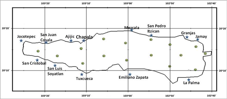
Sixteen sites (N = 16) were selected throughout the Lake Chapala area with the support of the Limnology Institute of the University of Guadalajara (Figure 1). In each site the DO concentration in five sections was quantified in situ; on the surface and at 1, 2, 3 and 4 m depth. We used 4 m as the maximum depth in this study since the average depth from 1934 to 2003 was 4.86 m (Hansen & van Afferden, 2004a), in addition we had the homogeneous data needed to make the model. The data used in this work were obtained in 1996-1997 in September, October, December, February and June covering the seasonal variability of rains, summer, and flow. In September, the largest amount of water from the Lerma River is collected, while in October the highest runoff from rainfall occurs. In December the flow decreases and there is growth of cyanophyte and Chlorophyceous algae. In February, the water inputs to the lake diminish, while June represents the end of the summer season with minimum levels of water as a response of little input and great extractions for agriculture and urban use.
Obtaining DO data
The data collection was performed by qualified personnel of the Institute of Limnology of the University of Guadalajara, using the electrometric method. For this analysis, a portable equipment containing a YSI Model 85 multiparameter glass electrode was used. This equipment was properly calibrated by the personnel in charge of the sampling.
Modeling of spatial variation
To determine the spatial variation of oxygen availability at different dates and depths, the interpolation technique known as ordinary kriging (OK) was used to generate the corresponding continuous surfaces (Burrough & McDonnell, 1998). Likewise, the standard errors corresponding to each sampling date were obtained. In this way, the variation was defined by anisotropic variograms (summary of the bivariate behavior of a randomized stationary function), which resulted in each sampling (by time and depth). Accordingly, experimental variograms were developed for each sampling date, which were used to model the spatial correlation between oxygen concentrations (Armstrong, 1998; Czaplewski, Reich, & Bechtold, 1994). The spatial variation defined by each experimental variogram was modeled based on the theoretical variogram that best defined the spatial continuity of the data. This is done with the purpose of estimating the values of variance at distances that are not covered by the experimental variogram (Flores & Moreno, 2005).
Validation criterion
To compare interpolations between different dates and depths, the cross-validation technique (Goovaerts, 1997), which consists of removing the sampled value of a particular site, after which its value is estimated based on the remaining sites (Isaaks & Srivastava, 1989). This is repeated for each site and then the actual and interpolated values are compared, and the differences are referred to as residuals, or errors (Flores and Moreno, 2005). A correlation analysis between the actual values and the estimated values allowed to evaluate the precision of the interpolations through the standard error (SE) of the prediction and the coefficient of determination. The SE allows us to weight the reliability of the regression equation, which is defined by correlating the actual values with the estimates values, as it measures the variability, or dispersion, of the observed values around the regression line.
Results
A first analysis of the data allowed us to determine if the level of DO along Lake Chapala was sufficient to sustain the biodiversity of the ecosystem, especially fish. In general, a concentration of 5 mg l-1 is considered adequate for this purpose, but if concentrations below 3 mg l-1 are present it may be lethal to wildlife (Iriondo & Mota, 2004; Rizo & Andreo, 2016). Figure 2 shows the DO variations, where the grid represents the resulting regression equation considering the location (length (X), latitude (Y)) and depth as independent variables. Except September and October sampling, the mean DO was greater than 5 mg l-1, with best availability in February, followed by December. In contrast, in October the southwest region of the lake has concentrations even lower than 3 mg l-1, which, as noted above, may affect the presence of fish in the area. The equations corresponding to the regressions of Figure 2 are presented in Table 1. It is remarked that the highest correlation was obtained for June and the lowest for December. In general, depth was the most significant variable (p < 0.05) in the DO concentration estimation, except October, where both coordinates predicted better concentration compared to depth. In the case of December only the length (X) was more significant than the depth.
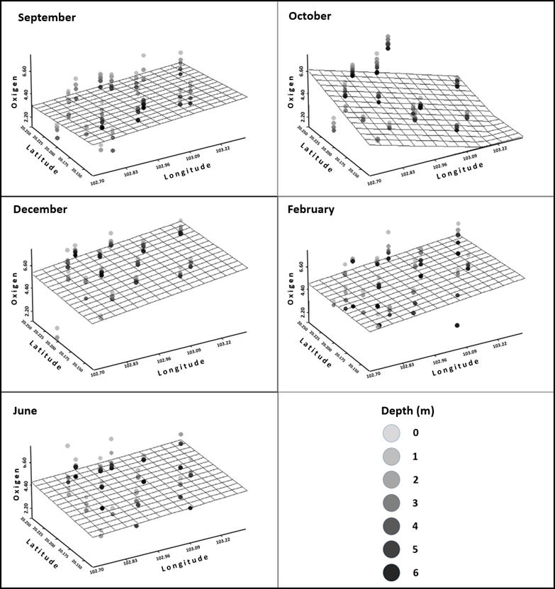
Figure 2 Modeling of the spatial variation of DO concentrations at different depths in Lake Chapala.
Table 1 Equations and statistics that correspond to the regression between oxygen and depth, for Lake Chapala.
| Date | Model | r2 | Pr(F) of X | Pr(F) of Y | Pr(F) of P |
|---|---|---|---|---|---|
| September | O = -115.2704 - 1.882943(X) - 3.639218(Y) + 0.5654791(P) | 0.4256 | 0.154 | 0.0775 | 0.0000 |
| October | O = -70.1952 + 3.7019(X) + 22.5058(Y) + 0.1851(P) | 0.4356 | 0.0000 | 0.0000 | 0.0345 |
| December | O = -635.7797 - 3.1648(X) + 15.6688(Y) + 0.7597(P) | 0.2018 | 0.0005 | 0.1555 | 0.0506 |
| February | O = -423.422 - 2.7406(X) + 7.2775(Y) + 0.1805(P) | 0.3495 | 0.0503 | 0.0898 | 0.0000 |
| June | O = -483.7652 - 3.4889(X) + 6.4927(Y) + 0.7616(P) | 0.5893 | 0.0004 | 0.6669 | 0.0000 |
| O = Oxigen (mg/l) | |||||
| X = Longitude coordinates (degrees) | |||||
| Y = Latitude coordinates (degrees) | |||||
| P = Depth (m) | |||||
Modeling of spatial continuity
Table 2 shows the models (spherical, linear and exponential) that were fitted to each variogram (Figure 3), as well as the three parameters that define its structure; nugget and sill range. In general, the results were similar, except variograms corresponding to depths of 3 and 4 m in September and depth of 3 m in February, whose SSR value was zero. This result implies that the variance of the sample explains the spatial variability of DO concentration. Based on these variograms, the maps that generate the temporal space variations of the DO are generated, which are analyzed, later (generation of continuous surfaces). On the other hand, the adjustment of the models varied from a r 2 of 0.00 to 0.966, which can be explained by the low number of sampling points. However, if a priori information is available, and the model that best fits the experimental variogram is sought, the criterion of r2 is adequate (Gallardo, 2006). However, it is preferred to use the residual squares (SQR), as a selection criterion, which represents a more robust measure of fit to the variogram data. Therefore, according to this parameter, the best results were found in October and June.
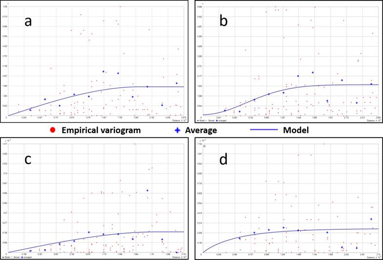
Figure 3 Variograms of DO concentrations in Lake Chapala, corresponding to September, for different depths: a) Surface, spherical model; b) 1 m, linear model: c) 2 m, spherical model; c) 3 m, linear model.
Table 2 Parameters and statistics of the models adjusted to the variograms of the oxygen concentration in Lake Chapala.
| DATE | DEPTH (m) | MODEL | Nugget | Sill | RANGE | SSR | r 2 OF VARIOGRAM MODEL | CROSS-VALIDATION | ||
|---|---|---|---|---|---|---|---|---|---|---|
| SQR | r 2 | EEP | ||||||||
| September | SURFACE | Spherical | 0.087 | 1.761 | 0.239 | 0.951 | 0.162 | 4.660 | 0.065 | 1.110 |
| -1 | Linear | 1.367 | 1.413 | 0.463 | 0.032 | 0.000 | 4.070 | 0.735 | 0.559 | |
| -2 | Spherical | 0.174 | 1.494 | 0.163 | 0.884 | 0.055 | 5.460 | 0.042 | 1.104 | |
| -3 | Linear | 2.307 | 2.307 | 0.452 | 0.000 | 0.738 | 7.620 | 0.960 | 0.326 | |
| -4 | Linear | 1.061 | 1.061 | 0.285 | 0.000 | 0.141 | 0.251 | 0.873 | 0.353 | |
| October | SURFACE | Spherical | 0.065 | 3.145 | 0.290 | 0.979 | 0.601 | 2.480 | 0.566 | 1.045 |
| -1 | Spherical | 0.395 | 3.410 | 0.313 | 0.884 | 0.512 | 3.820 | 0.455 | 1.221 | |
| -2 | Spherical | 0.620 | 3.448 | 0.299 | 0.820 | 0.464 | 3.860 | 0.441 | 1.259 | |
| -3 | Spherical | 1.158 | 4.035 | 0.348 | 0.713 | 0.839 | 0.452 | 0.393 | 1.363 | |
| -4 | Spherical | 1.900 | 7.809 | 0.609 | 0.757 | 0.966 | 0.148 | 0.360 | 1.657 | |
| December | SURFACE | Spherical | 0.250 | 6.686 | 1.059 | 0.963 | 0.116 | 69.000 | 0.121 | 1.251 |
| -1 | Spherical | 0.320 | 7.760 | 1.046 | 0.959 | 0.111 | 98.300 | 0.105 | 1.360 | |
| -2 | Exponential | 0.360 | 16.150 | 1.108 | 0.978 | 0.120 | 135.000 | 0.054 | 1.507 | |
| -3 | Spherical | 0.010 | 3.245 | 0.324 | 0.997 | 0.331 | 21.500 | 0.000 | 1.657 | |
| -4 | Exponential | 0.006 | 0.317 | 0.811 | 0.981 | 0.531 | 0.002 | 0.470 | 0.202 | |
| February | SURFACE | Spherical | 1.560 | 16.530 | 1.062 | 0.906 | 0.116 | 369.000 | 0.163 | 2.099 |
| -1 | Spherical | 0.010 | 12.320 | 1.071 | 0.999 | 0.170 | 181.000 | 0.332 | 1.427 | |
| -2 | Spherical | 0.700 | 7.871 | 1.281 | 0.911 | 0.224 | 47.700 | 0.111 | 1.576 | |
| -3 | Linear | 2.723 | 2.723 | 0.285 | 0.000 | 0.220 | 6.270 | 0.960 | 0.334 | |
| -4 | Spherical | 0.826 | 3.957 | 0.273 | 0.791 | 0.058 | 32.700 | 0.206 | 1.941 | |
| June | SURFACE | Linear | 0.001 | 3.011 | 0.945 | 1.000 | 0.405 | 2.400 | 0.498 | 0.592 |
| -1 | Linear | 0.001 | 2.011 | 0.846 | 1.000 | 0.709 | 0.584 | 0.568 | 0.468 | |
| -2 | Spherical | 0.272 | 2.033 | 1.143 | 0.866 | 0.568 | 0.753 | 0.067 | 0.503 | |
| -3 | Spherical | 0.910 | 5.854 | 0.620 | 0.845 | 0.595 | 1.940 | 0.079 | 1.772 | |
| -4 | Spherical | 2.401 | 4.803 | 0.768 | 0.500 | 0.362 | 0.767 | 0.283 | 1.378 | |
The results obtained during the modeling process (Table 2) show that the most homogeneous ratios in the explanation of variance (r2) correspond to the models of October and June data. However, the best fit (r = 0.96) was observed for models at a depth of 3 m in February and September. As for the standard error of prediction (SPE), it was similar in all models. In particular, the lower SPE values correspond to the models at depth 3 and 4 m (September); 4 m (December) and 3 m (February).
Generation of continuous surfaces
Based on the models obtained for each date and depth (Table 2) we defined the corresponding continuous surfaces that are exemplified in Figure 4, where we can observe how was the spatial variation DO in Lake Chapala. In general, minor concentrations were reported in September and October; however, the spatial variation was similar among the different depths in October, while the highest concentration corresponded to February. In October the highest concentrations were observed in the central and eastern regions of the lake, being similar in all depths.
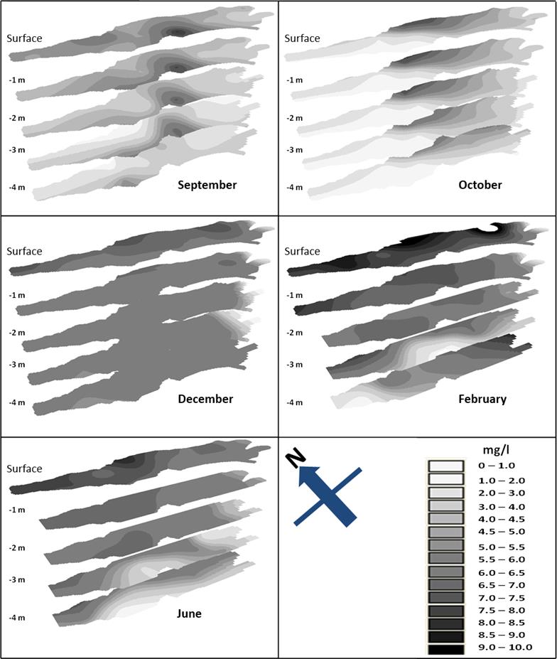
Figure 4 Spatial variation of DO concentrations in Lake Chapala, at different depths, corresponding to each sampling date.
Concerning December, the concentrations were rather similar at all depths, with a slight variation at the surface level. The highest DO concentration was found in the south-central region of the lake at all depths, except depth at 4 m, where a low concentration of oxygen was observed. The highest concentration was located on the surface, which decreased slightly in the east and west ends of the lake as the depth increased. In February, a lower concentration was observed at a depth of 3 m, which increased as the depth decreased, with the highest concentrations observed in the northern region of the lake. Finally, in June, although in lower concentrations, the major values were located in the northern part of the lake, observing notable variations in the different depths.
Correlation models
The equations corresponding to the regressions of Figure 2 are presented in Table 1. It is notorious that the highest correlation was obtained for June, the lowest being that of December. In general, depth was the most significant variable (p <0.05) in the estimation of DO concentration, except October, where both coordinates predicted better the concentration as compared to depth. In the case of December, only the length (X) was more significant than the depth.
Discussion
It is important to note that, despite its advantages, the use of the ordinary Kriging technique does not guarantee the best results in an interpolation (Flores & Moreno, 2005). That is, it is not possible to define a single interpolation technique that results in better estimates in all cases; however, the Kriging technique has detected minimal errors in some comparative studies and has therefore been considered the most appropriate (Dodd, Mechant, Rayner, & Morice, 2015). It is also important to specify that the spatial autocorrelation of a parameter is defined by several factors, such as sampling intensity, scale, distribution of sampling sites and differences between neighborhood values (Flores & Moreno, 2005). This implies that in a study of this type more than one interpolation technique could be tested. Also, the results also suggest, in all cases, that the number of sampling sites should be increased, since a smaller separation distance between sites defines better the trend of the spatial variability of these values (Flores, Reyes, & Moreno, 2004). Also, it is recommended that in future models, DO data obtained from other studies, performed in the study area, should be used. However, no studies were found that carry out a methodology similar to the one proposed in this study. Therefore, this work represents a first approximation to the described strategy. In this way, in future works it is suggested to incorporate data from other years, as well as to integrate auxiliary variables, to reinforce the estimates. Such spatial correlations are adequately defined through the technique of cokriging, which has the advantage of using the covariance of two or more related variables.
On the other hand, it is important to mention that even when it was possible to model using Ordinary Kriging, there are environmental factors and anthropogenic that modify so significant water quality. For example, the seasonal ones by the entrance of water during the rainy season, the existence of a period of recovery and temporary dynamics own ecosystem. This seasonal variation has been explained by various authors in different ecosystems. So, Rubio, Contreras, Quintana, Saucedo and Pinales (2012) detected seasonal differences in water quality of the Luis L. León dam in northern Mexico in nine quantified variables; while Rabee, Bahha and Ahmed (2011) observed these variations in a study conducted on the river Tigris in Iraq. Once the rains are over, the spatial distribution of the concentration of Oxygen is rather heterogeneous. This affirmation can be explained because the contribution of rain to the lake is not only from the main tributary (Lerma river) but of others. For example in October, the only source of water supply the lake comes from the Lerma River, observing increase in oxygen concentration in this zone. One possible explanation is that this is presents as a consequence of a process of re-alignment caused by the movement of water inflow (De la Mora, 2001; Lind & Dávalos, 2001). However, Simons (1984) showed that other variables have greater influence in the concentration of OD in the lake of Chapala, because after applying a model hydrodynamic observed that it is the wind, and not the flows of input and output the main factor that determines the patterns of water circulation. In his model he observed that with conditions normal wind from east to west at 9 km h-1, the flow of the Lerma River flows through the southern part from the lake to its middle part and the flow returns after this area. When the prevailing wind it is from west to east, the flow of water from the river Lerma runs through the middle part of the lake. This observed dynamics is an effective mechanism of transport of suspended materials and oxygen dissolved in the lake, which causes the Water column is in continuous motion, hence the little variability of its parameters physicochemical throughout the year. Also, due to the shallow depth of the lake and the mixture there is no seasonal stratification, but as is the case with other tropical lakes, there is a daily stratification when climatic conditions favor it (Lind & Dávalos, 2001). Normally the currents in the center of the lake are 0.1 km day-1 and in the zones of the banks is 0.5 km day-1. By orientation of the lake (from east to west), the of winds causes great waves and a body of completely mixed water (Lind & Dávalos, 2001). On the other hand, various studies have demonstrated that Lake Chapala presents problems of eutrophication since 1989, as result of the introduction of high concentrations of nutrients (Fernex et al., 2001; Waite, 1984). Since 1983, Lake Chapala presents an increase in the concentration of chlorophyll, which confers mesotrophic characteristics superior to eutrophic (Limón & Lind, 1990; Anda & Shear, 2001; Dávalos & Lind, 2001). In this sense, the importance of of the growth kinetics of the various organisms by the use of oxygen present in the water for the breathing of aquatic plants and plankton (Thomann & Mueller, 1987). In the results found in this work do not conditions of anoxia were recorded in the lake de Chapala, which coincides with other works (Quiróz, Mora, Molina, & García, 2004; Lara, 2014).
Conclusions
With this study, it was possible to model the spatial-temporal variation of DO concentrations, both along Lake Chapala and at different depths. In general, considering the DO as one of the main indicators of water quality, it was determined that the best quality water was concentrated in February and December, and according to the spatial result in the eastern part of the lake. However, it is important to note that, in spatial modeling, we try to define a model with the lowest estimation error considering the available variables. Therefore, in future studies, other strategies of interpolation could be tried where, among other aspects, the estimation of the spatial continuity could be improved if a greater intensity of sampling is considered; in particular, for those cases where the models do not fit well to the distribution of the variogram. It is also concluded that, although the interpolation allowed to define the spatial variation of the DO along the lake of Chapala, in the majority of the models the adjustment was low. That is, the results of the validation showed a low correlation between the observed and estimated values. This can be explained by the fact that, in some cases, the variograms presented a spatial tendency at the global level. The importance of the variogram analysis, prior to the estimation, is highlighted, where a more basic spatial analysis is suggested to evaluate the spatial autocorrelation of a given parameter, such as the Moran index (Reich & Geils, 1992). However, the results present important information so that, in subsequent studies, the way to include other elements for spatial modeling, such as, for example, environmental and anthropogenic factors, can be appropriately defined.
Referencias
Armstrong, M. (1998). Basic linear geostatistics. New York: Springer. [ Links ]
Bai, Q., Runling, L., Li, Z., Lepparanta, M., Arvola, L., & Li, M. (2016). Time-series analyses of water temperature and dissolved oxygen concentration in Lake Valkea-Kotinen (Finland) during ice season. Ecological Informatics, 36, 181-189. [ Links ]
Beltrán, R., Ramírez, J. P., & Sánchez, J. (2012). Comportamiento de la temperatura y el oxígeno disuelto en la Presa Picachos, Sinaloa, México. Revista Mexicana de Hidrobiología, 22, 94-98. [ Links ]
Burrough, P. A., & McDonnell, R. A. (1998). Principles of geographical information systems. Oxford, United Kingdom: Oxford University Press. [ Links ]
Czaplewski, R. L., Reich, R. M., & Bechtold, W. A. (1994). Spatial autocorrelation in growth of undisturbed natural pine stand across Georgia. Forest Science, 40, 314-328. [ Links ]
Dávalos, L., & Lind, O.T. (2001). Phytoplankton and bacterioplankton production and trophic relation in Lake Chapala (pp. 31-57). In: Hansen, A. M., & Van Afferden, M. (eds.), The Lerma Chapala watershed, evaluation and management. New York: Kluwer Academic/Plenum Publishers. [ Links ]
De-Anda, J., & Shear, H. (2001). Nutrients and eutrophication in Lake Chapala (pp. 183-198). In: Hansen, A. M., & Van Afferden, M. (eds.), The Lerma-Chapala watershed, evaluation and management. New York: Kluwer Academic/Plenum Publishers . [ Links ]
De-Jonge, V. N., Elliott, M., & Orive, E. (2002). Causes, historical development, effects and future challenges of a common environmental problem: eutrophication. Hydrobiologia, 1, 1-19. [ Links ]
De-la-Mora, C., Flores, J. G., Ruíz, J. A., & García, J. (2004). Modelaje estocástico de la variabilidad espacial de la calidad agua en un ecosistema lacustre. Revista Internacional de Contaminación Ambiental, 20(3), 99-108. [ Links ]
De-la-Mora, O. C. (2001). Evaluación de la calidad del agua del lago de Chapala durante 1996-1997. (Tesis de maestría). Zapopan, México: Universidad de Guadalajara. [ Links ]
Dodd, E. A., Mechant, Ch., Rayner, N., & Morice, C. (2015). An investigation into the impact of using various techniques to estimate arctic surface air temperature anomalies. Journal of Climate, American Meteorological Society, 2015, 1743-1763, DOI: http://dx.doi.org/10.1175/JCLI-D-14-00250.1. [ Links ]
Fernex, F., Zárate-del-V., P., Ramírez, H., Michaud, F., Parron, C., Dalmasso, J., Barci F., G., & Guzmán, M. (2001). Sedimentation rates in Lake Chapala (western Mexico): Possible active tectonic control: Chemical Geology, 177, 213-228. DOI: 10.1016/S0009-2541(00)00346-6. [ Links ]
Flores, J. G., & Moreno, D. A. (2005). Modelaje espacial de la influencia de combustibles forestales sobre la regeneración natural de un bosque perturbado. Agrociencia, 39(3), 339-349. [ Links ]
Flores, J. G., Reyes, O., & Moreno, D. A. (2004). Variación espacial del diámetro como respuesta a diferentes intensidades de muestreo en una cuenca forestal. Rev. Ciencia Forestal en México, 29(96), 47-66. [ Links ]
Gallardo, A. (2006). Geostadística. Ecosistemas, 15(3), 48-58. [ Links ]
Goovaerts, P. (1997). Geostatistics for natural resources evaluation. Applied geostatistics series. New York: Oxford University Press. [ Links ]
Hansen, A. M., & Van Afferden, M. (2004a). Modeling cadmium concentration in water of Lake Chapala, Mexico. Aquatic Sciences, 66, 266-273. [ Links ]
Hansen, A. M., & Van Afferden, M. (2004b). El agua de México visto desde la Academia. Jiménez, B., & Martín, L. (eds.). México, DF: Academia Mexicana de Ciencias. [ Links ]
Heddam, S. (2014). Modeling hourly dissolved oxygen concentration (DO) using two different adaptive neuro-fuzzy inference systems (ANFIS): A comparative study. Environmental Monitoring and Assessment, 186, 597-619. [ Links ]
Iriondo, A., & Mota, J. (2004). Desarrollo de una red neuronal para estimar el oxígeno disuelto en el agua a partir de instrumentación de EDAR. XXV Jornadas de Automática, Universidad de Castilla la Mancha, Ciudad Real, España, 8-10 de septiembre. [ Links ]
Isaaks, E. H., & Srivastava, R. M. (1989). An introduction to applied geostatistics. New York: Oxford University Press . [ Links ]
Lai, D. Y. F., & Lam, K. C. (2008). Phosphorus retention and release by sediments in the eutrophic Mai Po Marshes, Hong Kong. Marine Pollution Bulletin, 57, 349-356. [ Links ]
Lara, O. M. A. (2014). Aspectos ecológicos, cultivo, contenido de lípidos totales y proteínas del fitoplancton nativo de un lago polimíctico tropical (lago de Chapala). Tesis de maestría en Ciencias en Biosistemática y Manejo de Recursos Naturales y Agrícolas. Zapopan, México: Universidad de Guadalajara. [ Links ]
Limón, J. G., & Lind, O. T. (1990). The management of Lake Chapala, México. Lake Reservoir Management, 6, 61-70. [ Links ]
Lind, O. T., & Dávalos, L. (2001). An introduction to the limnology of Lake Chapala, Jalisco, Mexico (pp. 139-149). In: The Lerma-Chapala Watershed. Boston: Springer. [ Links ]
Mestre, R. J. E. (2011). La cuenca Lerma-Chapala, México. Estudio de caso VIII. Recuperado de http://www.bvsde.ops-oms.org/bvsacd/scan/033446/033446-18.pdf. [ Links ]
Nakova, E., Linnebank, F. E., Bredeweg, B., Salles, P., & Uzunov, Y. (2009). The river MESTA case study: A qualitative model of dissolved oxygen in aquatic ecosystems. Ecological Informatics, 4, 339-357. [ Links ]
Null, S. E., Mouzon, N. R., & Elmore, L. R. (2017). Dissolved oxygen, stream temperature, and fish habitat response to environmental water purchases. Journal of Environmental Management, 197, 559-570. [ Links ]
Olea, R. A. (1991). Geostatistical glossary and multilingual dictionary. New York: Oxford University Press . [ Links ]
Paéz, A., Alfaro, R., Cortés, R., & Segovia, N. (2013). Arsenic content and physicochemcial parameters of water from wells and termal springs at Cuitzeo Lake Basin, Mexico. International Journal of Innovative Research in Science, Engineering and Technology, 2, 12. [ Links ]
Paré, L. (1989). Los pescadores de Chapala y la defensa de su lago (144 pp.). Guadalajara, México: Instituto Tecnológico y de Estudios Superiores de Occidente. [ Links ]
Quiróz, C. H., Mora, Z. L. M., Molina, A. I., & García, R. J. (2004). Variación de los organismos fitoplanctónicos y la calidad del agua en el lago de Chapala, Jalisco, México. Acta Universitaria, 14(1), 47-58. [ Links ]
Rabee, A. M., Bahha, A. K., & Ahmed, A. (2011). Seasonal variations of some ecological parameters in Tigris River water at Baghdad region Iraq. J. Water Resources Protection, 3, 262-267. [ Links ]
Reich, R. M., & Geils, B. W. (1992). Review of spatial analysis techniques. Spatial analysis and forest pest management. USDA, FS. General Technical Report, 75, 142-149. [ Links ]
Rizo, L. D., & Andreo, B. (2016). Water quality assessment of the Santiago River and attenuation capacity of pollutants downstream Guadalajara City, Mexico. River Research and Application, 32, 1505-1516. [ Links ]
Rosales, L., Carranza, A., & López, M. (2000). Heavy metals in sediments of a large, turbid tropical lake affected by anthropogenic discharges. Environmental Geology, 39, 378-383. [ Links ]
Rubio, H., Contreras, M., Quintana, R. M., Saucedo, R., & Pinales, A. (2012). An overall water quality index (WQI) for a man-made aquatic reservoir in Mexico. International Journal of Environmental Research and Public health, 9, 1687-1698. [ Links ]
Samra, J. S., Gill, H. S., & Bhatia, V. K. (1989). Spatial stochastic modeling of growth and forest resource evaluation. Forest Science, 35, 663-676. [ Links ]
Sedeño, J. E., & López, E. (2007). Water quality in the Río Lerma, Mexico: an overview of the last quarter of the twentieth century. Water Resources Management, 21, 1797-1812. [ Links ]
Simons, T. J. (1984) Effect of outflow diversion on circulation and water quality of Lake Chapala. (Project MEX-CWS-010). Guadalajara, México: Centro de Estudios Limnológicos, Secretaría de Recursos Hidráulicos, Pan American Health Organization. [ Links ]
Singaraja, C., Chidambaram, S., Prasanna, M. V., Paramaguru, P., Johnsonbabu, G., & Thivya, C. (2011). A study on the behavior of the dissolved oxygen in the shallow coastal wells of Cuddalore District, Tamilnadu, India. Water Quality Exposure Health, 4(1), 1-16. [ Links ]
Thomann, R., & Mueller, J. (1987). Principles of surface water quality modeling and control. New York: Harper and Row, Publishers, Inc. [ Links ]
Trujillo, J. L., Saucedo, N. P., Zárate del V., P. F., Ríos, N., Mendizábal, E., & Gómez, S. (2010). Speciation and sources of toxic metals in sediments of Lake Chapala, Mexico. Journal of the Mexican Chemical Society, 54, 79-87. [ Links ]
United States Geological Survey, USGS (2013). United States Geological Survey. National field manual for the collection of quality-water data. Reston, USA: United States Department of the Interior, United States Geological Survey. [ Links ]
Waite, T. D. (1984). Principles of water quality. Orlando: Academic Press, Inc. [ Links ]
Wetzel, R. G. (2001). Limnology: Lake and river ecosystems. San Diego: Academic Press. [ Links ]
Wu, Y., Wen, Y., Zhou, J., & Wu, Y. (2014). Phosphorus release from lake sediments: Effects of pH, temperature and dissolved oxygen. Journal of Civil Engineering, 18, 323-329. [ Links ]
Yuan, L. L., & Pollard, A. I. (2015). Classifying lakes to quantify relationships between epilimnetic chlorophyll a and hypoxia. Environmental Management, 55, 578-587. [ Links ]
Zhai, S., Yang, L., & Hu, W. (2009). Observations of atmospheric nitrogen and phosphorus deposition during the period of algal bloom formation in northern lake Taihu, China. Environmental Management, 44, 542-551. [ Links ]
Zhang, Y., Wu, Z., Liu, M., He, J., Shi, K., Zhou, Y., Wang, M., & Liu, X. (2015). Dissolved oxygen stratification and response to thermal structure and long-term climate change in a large and deep subtropical reservoir (Lake Qiandaohu, China). Water Research, 75, 249-258. [ Links ]
Received: January 19, 2017; Accepted: July 17, 2017
 Este es un artículo publicado en acceso abierto bajo una licencia
Creative Commons
Este es un artículo publicado en acceso abierto bajo una licencia
Creative Commons
