


Services on Demand
Journal
Article
 text in
  English (pdf)
 Article in xml format
 Article references
 Send this article by e-mail
Indicators
-
 Cited by SciELO
 -
 Access statistics
Related links
-
 Similars in
SciELO
Similars in
SciELO
Share

 Permalink
Revista mexicana de ciencias forestales
Print version ISSN 2007-1132
Rev. mex. de cienc. forestales vol.10 n.53 México May./Jun. 2019
https://doi.org/10.29298/rmcf.v10i53.500
Articles
A generalized nonlinear height-diameter model with mixed-effects for seven Pinus species in Durango, Mexico
1Instituto Tecnológico de El Salto. México.
2Programa de Maestría en Ciencias en Desarrollo Forestal Sustentable. Instituto Tecnológico de El Salto. México.
3Campo Experimental Valle del Guadiana. Instituto Nacional de Investigaciones Forestales, Agrícolas y Pecuarias. México.
Durango is the major state for timber production in Mexico (28.5 % of the national total); it is estimated that the area under use is 2 million hectares, which is why forest management is an important task for forestry managers. The height-diameter relationship (h-d) is mainly used to describe the structure of a stand, to estimate the individual-tree total volume or stand level volume and to assess the site quality. In this study, a generalized equation was developed for the h-d relationship of seven conifer species in mixed-species forests in northwestern Durango, Mexico. The equation considers diameter at breast height, dominant height, stand basal area and density as independent variables. The nonlinear mixed effect model procedure was used to fit data coming from 44 permanent sample stem-mapped plots. The generalized model explained 82 % of the total variability. Model calibration involved measuring the tree total height in a sample of three trees of average diameter class for each plot. The equation developed could be used as a biometric tool for forest management in mixed forests of the study area.
Key words: Mixed-species forests; calibration process; generalized equation; non-linear mixed models; Pinus sp.; height-diameter relationship
Durango es el principal estado en México para la producción de madera (28.5 % del total nacional). Se estima que la superficie bajo aprovechamiento es de 2 millones de hectáreas; razón por la cual, la ordenación forestal es una tarea importante para los manejadores silvícolas. El conocimiento sobre la relación altura-diámetro (h-d) de los árboles se utiliza, principalmente, para caracterizar la estructura del rodal, estimar el volumen de los árboles individuales o del rodal, y para determinar la altura dominante con el propósito de evaluar la productividad vía el índice de sitio. En este trabajo se desarrolló una ecuación generalizada para describir la relación h-d de siete especies de coníferas en los bosques mezclados del noroeste de Durango, México. La ecuación considera como variables independientes al diámetro normal, altura dominante, área basal y la densidad. Para la variabilidad entre 44 sitios permanentes, el ajuste de la mejor ecuación fue mediante el enfoque de modelos mixtos no lineales. El modelo generalizado desarrollado explicó 82 % de la variabilidad total de los datos observados. Para calibrar el modelo mixto se determinó que se requiere medir la altura total de una submuestra de tres árboles de clase diamétrica promedio dentro de cada parcela. La ecuación generada constituye una herramienta para el manejo forestal de los bosques mezclados del área de estudio.
Palabras clave: Bosques mezclados; calibración; ecuación generalizada; modelos mixtos no-lineales; Pinus sp.; relación altura-diámetro
Introduction
Forest management in Mexico requires quantitative prediction mechanisms that provide detailed information on the growth and development of natural forests. In modern management, framed in the concept of sustainability, it is necessary to improve the precision in the design of silvicultural prescriptions that can only be provided by tools that involve the variables of the stand (Vargas et al., 2017). Total height estimation (h) of the trees in a stand has two roles in the modeling of growth and production: (1) dominant height and age, used to estimate the productivity of the site; (2) height-diameter curves, which are the basis for predicting the total and commercial volumes of tree and the forest stand (López et al., 2003). Accurate estimation of the h-d ratio is important because total height is a more difficult and expensive variable to measure in the field than normal diameter, and is usually measured only in a sample of trees (Sharma and Breidenbach, 2015).
The height-diameter relationship (h-d) can be adjusted with linear and non-linear functions (Huang et al., 1992). The relationships that consider only the normal diameter, known as local functions, do not adapt well to all possible conditions of forest growth and different silvicultural status of the stands, because total height varies with the quality of the season or with density (Prodan et al., 1997). Therefore, a single function cannot be used to estimate all the possible h-d relationships which can be found within the different stands throughout their development; for this reason, to improve accuracy, variables that characterize the dynamics of each stand must be included, giving rise to the so-called generalized functions (Crecente et al., 2010; Hernández et al., 2015).
Total height, as well as normal diameter are obtained from trees of the same sampling site, which are found in masses at different geographical locations, so that such data has a hierarchical structure, since data from the same sampling unit tends to look alike. This nested stochastic structure results in a lack of measurement independence, since observations on each sampling site may be correlated (Gregoire, 1987; Fox et al., 2001).
Mixed effects models have been used successfully to treat these types of problems (Calama and Montero, 2004; Castedo et al., 2006); this technique estimates, simultaneously, fixed (common for the population) and random (specific for each site) parameters in the same model and allows modeling the variability detected between sites of the same sample or population, which makes them more efficient to predict the total height of a new tree. In addition, the inclusion of specific random parameters for each sampling site within the model explains the variability of a given phenomenon among its different locations (after defining the structure of the variances-covariance matrix of random parameters), providing an improvement in the estimates of the dependent variable (total height of the tree) (Castedo et al., 2006).
Durango is the most important state for the production of wood (28.5 % of the national total) in Mexico and it is estimated that the area under use is 2 million hectares (Luján et al., 2016), which is why forest management is an important task for silvicultural managers. In the Sierra Madre Occidental in Durango, the predominant vegetation types are pine-oak stands, often mixed with Pseudotsuga, Arbutus and Juniperus. Pinus species account for about 80 % of all timber production followed by of the genus Quercus (Návar et al., 2013).
Thus, an efficient h-d function for mixed forests proves its usefulness when included in the growth and production models used in forest management; in addition, it is a good tool for estimating total height of trees in the site from a sub-sample taken in the field, saving time and cost in timber inventories (Vargas et al., 2009; Corral et al., 2014, Guerra et al., 2019).
Based on these considerations, the purpose of this work was to develop a generalized equation to efficiently describe the h-d relationship with estimated parameters by fitting mixed-effect models for seven conifer species from the northwestern region of Durango state.
Materials and Methods
Study area
The study was conducted in mixed forests of the San Diego de Tezains and Salto de Camellones ejidos which belong to the Forestry Management Unit (UMAFOR) 1005 "Santiago Papasquiaro y Anexos". The study area is located in the northwest region of the state of Durango, Mexico, between 24°30'-25°27' N and 105°01'-106°24' W. Height above sea level fluctuates between 800 and 3 103 m. The prevailing climate is temperate with rain in summer. The average annual rainfall varies from 1 000 to 1 200 mm. The average annual temperature fluctuates from 5 to 18 °C, the coldest temperature occurs in January (-6 °C) and the hottest in May (28 °C) (García, 1981; Quiñonez et al., 2018). The most important forest communities are made up of species of Pinus, Quercus, Juniperus, Cupressus, Pseudotsuga, Arbutus and Alnus. Approximately 90 % of the study area consists of mixed stands with irregular structures (Quiñonez et al., 2018).
Source of the data
The mensuration information used to adjust the functional relationship h-d was obtained from 44 units or permanent sampling sites and monitoring of growth and production, established in 2008, covering all types of vegetation, site qualities, densities and ages in the stands in timber production. The dimensions of the sites are 50 × 50 m and they were established under a systematic sampling design. For each tree with a normal diameter equal to or greater than 7.5 cm, information was recorded on species, normal diameter (d, cm), total height of the tree (h, m), crown diameter (m) and its position with respect to the center of the plot (azimuth, degrees, distance, m).
A database with a total of 24 species was processed. The estimated composition was 84 % for the genus Pinus (P. arizonica Engelm., P. ayacahuite Ehrenb., P. durangensis Martínez, P. herrerae Martínez, P. lumholtzii B.L. Rob. & Fernald, P. teocote Schiede ex Schltdl. & Cham., P. douglasiana Martínez), 8 % for the genus Quercus (Q. sideroxyla Humb. & Bonpl., Q. arizonica Sarg., Q. mcvaughii Spellenb, Q. durifolia Seemen ex Loes, Q. crassifolia Bonpl., Q. jonesii Trel., Q. rugosa Neé, Q. laeta Liebm.) and 8 % for species of the genus Juniperus, Cupresus, Arbutus and Alnus (J. deppeanna Steud., J. durangensis Martínez, C. lusitanica Mill., A. arizonica (A. Gray) Sarg., A. bicolor M. González & PD Sørensen, A. madrensis M. González, A. tesselata PD Sørensen, A. xalapensis Kunth., and Alnus firmifolia Mill). Only the h-d data of Pinus species were used. The distribution of the pairs of data was examined through graphs to detect outliers, which were eliminated from the database used for equation adjustment, the main descriptive statistics of the variables analyzed are shown in Table 1.
Table 1 Descriptive statistics of the variables used in the adjustment of h-d equations.
| Species | Number of trees | d (cm) | h (m) | ||||||
|---|---|---|---|---|---|---|---|---|---|
| Minimum | Maximum | Average | SD | Minimum | Maximum | Average | SD | ||
| P. arizonica | 205 | 7.5 | 52.0 | 19.3 | 10.9 | 2.8 | 29.3 | 13.4 | 6.2 |
| P. ayacahuite | 281 | 7.5 | 91.3 | 15.2 | 9.6 | 2.3 | 38.1 | 9.7 | 4.4 |
| P. durangensis | 1730 | 7.1 | 99.5 | 17.0 | 10.6 | 2.9 | 35.3 | 11.9 | 5.5 |
| P. herrerae | 629 | 7.3 | 78.5 | 22.6 | 13.6 | 2.9 | 35.3 | 15.6 | 6.5 |
| P. lumholtzii | 287 | 7.5 | 46.5 | 16.9 | 7.1 | 2.3 | 23.6 | 10.4 | 4.7 |
| P. teocote | 803 | 6.9 | 68.0 | 17.5 | 10.1 | 2.7 | 34.7 | 10.9 | 4.8 |
| P. douglasiana | 98 | 7.5 | 79.3 | 18.1 | 13.2 | 3.7 | 25.1 | 11.6 | 5.6 |
| Pinus sp * | 4033 | 6.9 | 99.5 | 18.0 | 11.0 | 2.3 | 38.1 | 12.1 | 5.7 |
SD = Standard deviation of the mean; * = It includes the entire database of the genus Pinus.
The following indicators were estimated for each sampling unit (site): the number of trees per hectare (N, trees ha-1), basal area per hectare (G, m2 ha-1), mean square diameter (dg, cm), dominant height estimated as the average of the 25 trees with the largest diameter in the plot (H 0 , m) (Assmann, 1970), dominant diameter estimated as the average of the 25 trees with the largest diameter in the plot (D 0 , cm) (Assmann, 1970) and Hart Index (%) estimated by the expression:
Models
Ten local equations and 10 generalized equations were analyzed and compared to describe the h-d relationship (Table 2). The adjustments were individual, by species and in group (all species of the genus Pinus) by ordinary non-linear least squares (ONLS) with the R program (R Core Team, 2016) by means of the "nlsLM" function of the "minpack.lm" package (Elzhov et al., 2012).
Table 2 Local and generalized h-d equations analyzed.
| (Equation) Reference | Expression |
|---|---|
| Local | |
| (1) Bates y Watts (1980) |
|
| (2) Burkhart y Strub (1974) |
|
| (3) Meyer (1940) |
|
| (4) Stage (1975) |
|
| (5) Huang et al. (1992) |
|
| (6) Huang et al. (1992) |
|
| (7) Wykoff et al. (1982) |
|
| (8) Chapman-Richards (Uzoh, 2017) |
|
| (9) Hossfeld (1822) |
|
| (10) Weibull (1951) |
|
| Generalized | |
| (11) Sharma y Parton (2007) |
|
| (12) Cox I (López et al., 2003) |
|
| (13) Cox II (López et al., 2003) |
|
| (14) Sharma and Parton (2007) |
|
| (15) Schröder and Álvarez I (López et al., 2003) |
|
| (16) Schröder and Álvarez II (López et al., 2003) |
|
| (17) Mirkovich (1958) |
|
| (18) Harrison (López et al., 2003) |
|
| (19) Pienaar (López et al., 2003) |
|
| (20) Hui and Gadow (López et al., 2003) |
|
h = Total height (m); d = Normal diameter (cm); H 0 = Dominant height (m); D 0 = Dominant diameter (cm); N = Density (number of trees ha-1); G = Total basal area (m2 ha-1); d g = Mean square diameter (cm); ln = Natural logarithm; b i = Estimated parameters.
Adjustment capacity evaluation was based on residual graphs, numerical comparisons of the root mean square error (RMSE), values of the coefficient of determination (R 2 ), the average bias of the residuals (Em) and Schwarz Baysian Information Criterion (BIC) (Schwarz, 1978) which compares equations in terms of their parsimony (simplicity). The formulation of these statistics is expressed as follows:
Where:
n = Number of observations
k = Number of parameters of the equation
ln = Natural logarithm
For local equations which showed the greatest advantage in goodness-of-fit-statistics, the relationship between the parameters and the site variables (covariables) was analyzed, in order to better explain the variability between total height and the characteristics of the variables. For the inclusion of covariates in the base model, different combinations of stand variables and their transformations (square, logarithm, root, inverse, etc.) were also tested in order to improve the adjustments. The relationship was analyzed through the "cor" function of R (R Core Team, 2016) and graphical analysis.
Mixed-effects model
While the h-d data pairs used in fitting the equations were obtained from different sampling units, a high correlation was detected between the measurements taken within the sampling unit, which infringes one of the fundamental assumptions of the regression model. In order to deal with the lack of independence between observations, the mixed-effects model was used, in which the variability between sampling units is explained by the introduction of a random parameter that is estimated together with the fixed parameters (Pinheiro and Bates, 1998; Calama and Montero, 2004; Castedo et al., 2006).
The parameters vector in a non-linear mixed model can be defined, according to Pinheiro and Bates, (1998) in the following way:
Where:
f = Non-linear function
Vector
Where:
λ = px1 vector for the fixed parameters (p being the number of fixed parameters)
bi = qx1 vector for the random parameters, related to the ith unit (q is the number of random parameters)
Ai and Bi = rxp and rxq size matrixes for the fixed and random effects, respectively, corresponding to the ith unit
The basic theoretical assumptions of the non-linear mixed models assume that the residual vector (εi ) and the random effect vector (bi) have a normal distribution, with mean equal to zero and a variance-covariance matrix (Ri and D) which represents the variability between the different sampling units (Littell et al., 2006).
Random Parameters Estimation
The random parameters were estimated using the maximum likelihood marginal approximation of the empirical best linear unbiased predictor (EBLUP) (Vonesh and Chinchilli, 1997) from the expansion of the Taylor serie, using the algorithm of Lindstrom and Bates (1990), implemented in the "nlme" function of R (R Core Team, 2016).
The construction of the generalized equation with mixed effects inclusion was based on the selection of the local equation which showed the best goodness-of-fit results of all of the species under study. Thus, different combinations of fixed and random parameters were tested in each equation, and the RMSE, R2 , Em and BIC statistics were compared in order to determine which fixed parameters should be considered as mixed. The h-d equation generated in this way was compared with the best generalized equation.
Random parameters prediction
The application of the mixed effects model requires previous information on the response variable (total tree height) that is later used to calculate the specific random parameters of that sample unit. The measured heights of one or more trees at each site can be used to predict the specific random parameters for that sampling unit and adjust the fixed part of the mixed effects model (average population response) to the stand conditions. This is known as location or calibration of the mixed effects model (Sharma et al., 2016).
When a sub-sample of mj tree heights is available, it can be used to predict the random parameters of vector bj, with the following equation (Vonesh and Chinchilli, 1997):
Where:
To determine the optimal size of the sub-sample of trees to be measured within each sample unit and find the response of the calibration (RC), the following options were analyzed:
RC1: Measure the total height of a tree and the minimum normal diameter of each sample unit
RC2: Measure the total height of two trees, together with the minimum and average normal diameter of each unit
RC3: Measure the total height of three trees together with the minimum, average and maximum normal diameter of each unit
RC4: Measure the total height of a middle class tree (selected as the average between the minimum normal diameter and the average normal diameter of each unit)
RC5: Measure the total height of two middle class trees (selected as the average between the minimum normal diameter and average normal diameter and, average between the average normal diameter and the maximum normal diameter of each unit)
RC6: Measure the total height of three middle class trees (selected as the average normal diameter and the two trees selected in the RC5 option in each unit)
The six alternatives described were evaluated in terms of RMSE, R2 and Em and compared with the statistics obtained by the equations adjusted with the ONLS and NLME procedure (i.e. when all the trees in the unit are included).
Heights of trees predictions in the different calibration options evaluated were calculated with the method used to estimate the random parameters through the following expression:
Where:
Results and Discussion
Local and generalized equations
To select the local and generalized equation with the best individual goodness-of-fit result for each species, firstly, all equations in Table 2 were adjusted by species. During this stage, convergence problems and non-significant parameters were identified for some of them (Pinus ayacahuite, P. herrerae, P. lumholtzii and P. douglasiana) with equations (10), (13) and (17); after that, it was decided to carry out the subsequent analyzes with the joint database for all Pinus genera.
When comparing the values of goodness-of-fit statistics for the group of local equations (Table 3), Equations (3), (8), (9) and (10) were the most accurate and with the least bias. Although these four equations provided very similar values in the comparison statistics used, equation (3) presented non-significant parameters in the fit, even though the BIC value was slightly lower than the rest of the equations. Finally, the graphical bias analysis in height estimation by diametric classes indicated that equation (8) showed the best behavior in the whole data interval, so it was selected as the base model to study the inclusion of variables of stand in its structure (Figure 1a).
Table 3 Goodness-of-fit statistics values of local and generalized equations adjusted to h-d data from seven Pinus genus species.
| Ecuación | Locales | Ecuación | Generalizadas | ||||||
|---|---|---|---|---|---|---|---|---|---|
| RMSE | R 2 | Em | BIC | RMSE | R 2 | Em | BIC | ||
| (1) | 2.95 | 0.731 | -0.011 | 20 298 | (11) | 2.44 | 0.816 | -0.017 | 18 680 |
| (2) | 3.11 | 0.701 | 0.099 | 20 616 | (12) | 2.86 | 0.747 | -0.100 | 19 965 |
| (3) | 2.95 | 0.731 | -0.001 | 20 192 | (13) | 2.42 | 0.819 | 0.006 | 18 652 |
| (4) | 2.99 | 0.724 | -0.038 | 20 297 | (14) | 2.45 | 0.815 | -0.020 | 18 713 |
| (5) | 2.96 | 0.730 | -0.017 | 20 208 | (15) | 2.47 | 0.812 | -0.006 | 18 767 |
| (6) | 3.64 | 0.590 | -0.173 | 21 897 | (16) | 2.46 | 0.813 | -0.007 | 18 755 |
| (7) | 3.07 | 0.709 | 0.085 | 20 516 | (17) | 2.55 | 0.799 | 0.045 | 19 028 |
| (8) | 2.95 | 0.731 | 0.004 | 20 200 | (18) | 2.52 | 0.804 | -0.013 | 18 933 |
| (9) | 2.95 | 0.731 | 0.004 | 20 200 | (19) | 2.52 | 0.804 | 0.066 | 18 916 |
| (10) | 2.95 | 0.731 | 0.004 | 20 200 | (20) | 2.51 | 0.805 | -0.045 | 18 911 |
RMSE = Root mean square error; R 2 = Coefficient of determination; Em = Average bias; BIC = Schwarz Bayesian information criterion.
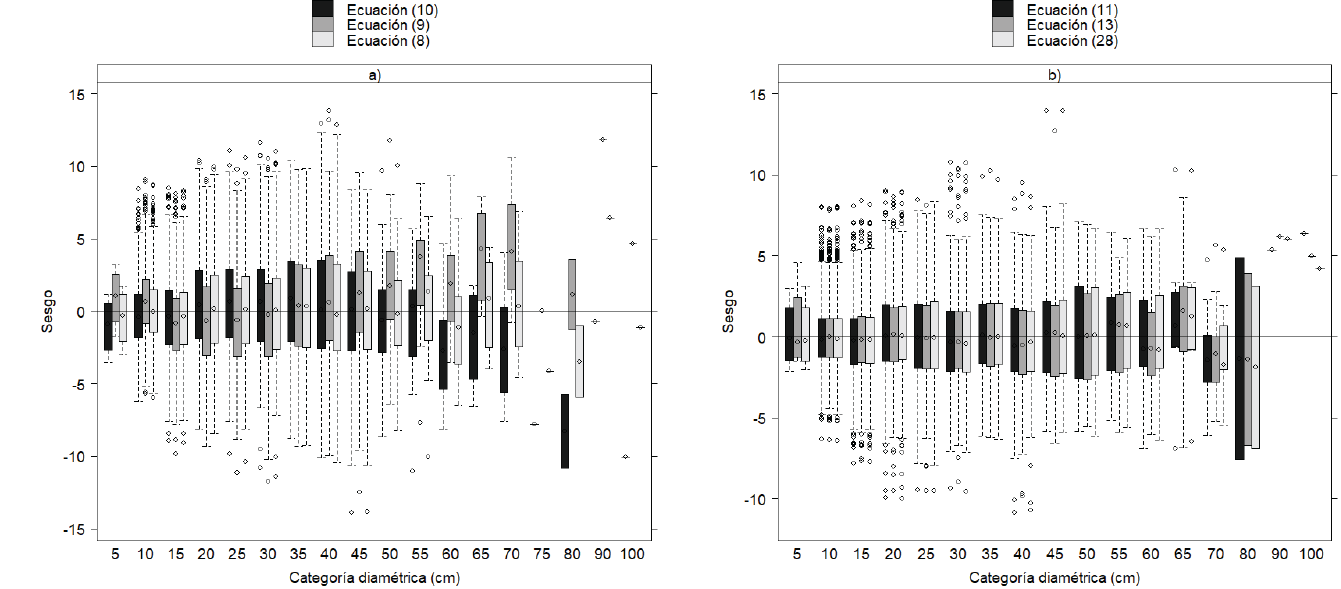
Figure 1 Bias behavior by diametric class of local and generalized equations with the best goodness-of-fit results.
Huang et al. (2000) and Peng et al. (2001) point out that Equation (8) is perhaps the most flexible and versatile to model the h-d relationship in forest stands. In this regard, Uzoh (2017) showed that the Equation (8) of Chapman-Richards is statistically the most robust (i.e. least biased) out of 12 different options to estimate the height of Pinus ponderosa Douglas ex Lawson in a mixed-effects model in the west of the United States of America.
While comparing the goodness-of-fit statistics values of the generalized equations group (Table 3), equations (11) and (13) stand out as the most accurate, considering R2 and RMSE statistics. However, Equation (13) exhibited non-significant parameters, even though it has the lowest value in BIC results. Therefore, the generalized equation of Sharma and Parton’s (2007) (11) was that of the best advantages in precision and parsimony (BIC) of all evaluated equations. In addition to this, the graphical analysis of bias while estimating heights by diameter classes had an unbiased behavior (Figure 1b). This equation is quite flexible to describe the h-d relationship and has been widely used in similar studies (Vargas et al., 2009; Crecente et al., 2010; Corral et al., 2014).
The best goodness-of-fit statistics in terms of precision and parsimony are derived from the generalized equations (Table 3), since they include stand characteristics as predictor variables, which decrease variability within each sample unit, and in general, are widely recommended to describe the h-d relationship (López et al., 2003; Barrio et al., 2004; Canga et al., 2007; Vargas et al., 2009; Crecente et al., 2010; Corral et al., 2014; Uzoh, 2017).
The correlation analysis between stand variables and the parameters in Equation (8) (Table 4) show that only three variables (H0 , N and G) were significantly correlated to improve their accuracy, resulting in the generalized equation with the following expression:
Where:
b0 - b4 = Parameters of the equation; the rest of the previously defined variables
Table 4 Correlation between the estimators of Equation (8) and stand variables.
| Variable | b 0 | b 1 | b 2 | N | G | d g | H 0 | D 0 | IH |
|---|---|---|---|---|---|---|---|---|---|
| b 0 | 1.00 | ||||||||
| b 1 | -0.51 | 1.00 | |||||||
| b 2 | 0.32 | -0.50 | 1.00 | ||||||
| N | 0.32 | -0.05 | 0.41 | 1.00 | |||||
| G | 0.46 | -0.31 | 0.35 | 0.60 | 1.00 | ||||
| d g | 0.10 | -0.14 | -0.59 | -0.58 | 0.11 | 1.00 | |||
| H 0 | 0.47 | -0.38 | 0.08 | 0.23 | 0.79 | 0.46 | 1.00 | ||
| D 0 | 0.50 | -0.38 | -0.01 | 0.13 | 0.76 | 0.61 | 0.87 | 1.00 | |
| IH | -0.42 | 0.16 | -0.30 | -0.65 | -0.72 | 0.06 | -0.72 | -0.60 | 1.00 |
Where:
H0 = Dominant height (m)
D0 = Dominant diameter (cm)
N = Density (number of trees ha-1)
G = Total basal area (m2 ha-1)
dg = Mean square diameter (cm)
IH = Hart Index (%)
bi = Estimated parameters
With the inclusion of dominant height, basal area and stand density, in addition to normal diameter in Equation (28), RMSE was reduced by 18 % with respect to the Chapman-Richards base model (Equation 8) (from 2.95 m to 2.43 m) and, consequently, R2 was increased by 12 % (from 0.731 to 0.818). BIC was reduced by 8 % (from 20 200 to 18 651) since it includes the sum total of the residual squares.
On the other hand, while comparing the precision and parsimony of Equation (28) with respect to Equation (11), developed by Sharma and Parton (2007), a marginal improvement was also found since RMSE decreased by 0.4 % and the value of R2 increased by 0.16 %, while BIC had a reduction of 1.5 %.
Based on goodness-of-fit statistics and on the graphical behavior of bias by diametric class (Figure 1b), Equation (28) was taken as base model to adjust it using the mixed effects technique in the h-d ratio of the seven species under study. This equation includes dominant height as an indicator of productivity, basal area as a simple and objective measure of trees occupancy and that in general is better than the number of trees per hectare, since it combines the number of trees with its size (Huang et al., 2009), and the number of trees generates predictions subject to instantaneous changes according to the thinnings or silvicultural interventions to which the masses are subjected (Crecente et al., 2010). These variables have been used in modeling the h-d relationship by different authors for a wide variety of species (López et al., 2003; Calama and Montero, 2004;Canga et al., 2007; Crecente et al., 2010; Corral et al., 2014; Sharma and Breidenbach, 2015).
Mixed effects model
While adjusting Equation (28), it became clear that the parameters with the greatest variability were those that define the asymptote and the shape of the h-d curve (Table 5). Therefore, in a first step it was adjusted with the parameters that define the asymptote (b0 , b1 ) and the form (b3 , b4 ) as random; however, since no convergence was found, several combinations were tested with one and two random parameters associated with the fixed parameters until convergence was achieved.
The best combination was found by associating the shape parameter (b3 ) with a random parameter ui in an additive way (b3 + ui ). Similar results have been reported by Sharma and Parton (2007), Vargas et al. (2009) and Corral et al. (2014), who considered only one random parameter within the mixed model.
The generalized final model with mixed effects is expressed as follows:
Where:
b0 - b4 = Fixed parameters (common to all sample units)
The mixed effects model (Equation 29) showed an improvement in precision of 6.6 % in RMSE value with respect to the base model (Equation 28); in addition to this, with the inclusion of the random parameter among the sample units, a 2.8 % increase on the value of R2 was achieved, explaining the observed variability. On the other hand, the value of the average bias in both equations was similar, but BIC, which evaluates the simplicity of the model, was reduced by 2.9 % (Table 5).
Table 5 Parameters and goodness-of-fit statistics of the base and mixed effects models applied.
| Parameters | Base Model Equation (28) |
Mixed Effects Model Equation (29) |
|---|---|---|
| Fixed parameters | ||
| b 0 | 3.131 | 7.689 |
| b 1 | 1.858 | 1.324 |
| b 2 | 0.031 | 0.029 |
| b 3 | 1.017 | 1.023 |
| b 4 | 0.071 | -0.023 |
| Variance components | ||
| σ2 | 5.196 | |
| σ2 u | 0.011 | |
| Goodness-of-fit | ||
| RMSE | 2.430 | 2.270 |
| R 2 | 0.818 | 0.841 |
| Em | -0.009 | -0.009 |
| BIC | 18651 | 18 101 |
Figure 2a shows residual dispersion against heights predicted by (Equation 29); a homogeneous variance is observed throughout the data interval, and there is no systematic pattern in the variability of residuals. Therefore, the random effect helped eliminate heterogeneity in the variance (Fang and Bailey, 2001). On the other hand, the graph of residuals against first delay (Figure 1b) does not indicate an autocorrelation tendency, which means that it was removed when the random effect among sample units was modeled by expanding parameter b3.
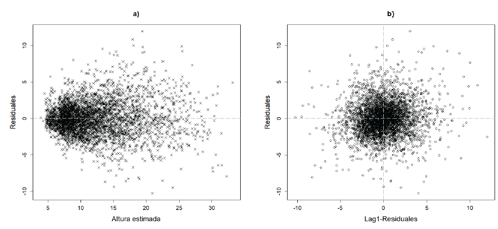
Figure 2 Residuals against the predicted heights (a), residuals versus the first delay (b) estimated with Equation 29.
Model Calibration
The results of calibration alternatives to improve predictions are shown in Table 6. The highest values of RMSE were obtained by including a subsample of one to three trees with extreme diameter categories (minimum and maximum). In contrast, with the inclusion of trees belonging to central diametric categories, a slight reduction in RMSE was identified. Although there is no methodology for defining the most appropriate sample size in the calibration of a mixed-effects model, it is noted that the RC6 alternative was found to be more accurate while measuring total height in a subsample of three randomly selected trees with diameters close to the second quartile of the site’s diametric structure, given that it presented a 4.6 % reduction in RMSE in regard to the estimated value during the adjustment of Equation (28) by ONLS. This value was very close to the one generated with the mixed effects model adjustment (measurement of the total height of all trees) of (Equation 29) by NLME procedure.
Table 6 Comparison of RMSE calibration alternatives of Equation (29).
| Calibration alternatives | RMSE | % RMSE reduction |
|---|---|---|
| Equation 28 (ONLS) | 2.430 | -- |
| Equation 29 (NLME) | 2.270 | -6.6 |
| RC1 (height of 1 tree) | 2.454 | 1.0 |
| RC2 (height of 2 trees) | 2.449 | 0.8 |
| RC3 (height of 3 trees) | 2.461 | 1.3 |
| RC4 (height of 1 tree) | 2.428 | -0.1 |
| RC5 (height of 2 trees) | 2.424 | -0.2 |
| RC6 (height of 3 trees) | 2.319 | -4.6 |
The mixed effects model registered an increase in accuracy, because it includes the variability that exists in the total height of trees within and between plots (Calama and Montero, 2004). Given that mixed forests have a greater variability in total tree height compared to those that come from stands with one or two species, it is estimated that the predictions of the developed mixed effects model is acceptable, since it explains 82 % of the data variability. In experiences with data from regular masses, a close to 90 % prediction capacity has been achieved (Calama and Montero, 2004; Diéguez et al., 2005; López et al., 2012).
The calibration of mixed-effects models is an advantage for forest managers, since it is possible to determine the height of all the trees in the stand from only a few trees. Calama and Montero (2004) propose four randomly selected trees; Corral et al. (2014) define that three trees close to 10 % of the average diameter are sufficient, while Castedo et al. (2006) and Crecente et al. (2010) propose the three smallest trees of the stand's diametric structure. As the number of trees selected to calibrate a mixed-effect model increases, RMSE is generally reduced and the predictive capacity of the model is improved. However, this is not always justified since the cost of sampling increases, so calibration with a small sample of trees is the main advantage of the mixed effects models when applied in the forest field (Castedo et al., 2006).
Conclusions
Using a generalized equation, the h-d relationship was described based on the Chapman-Richards growth model, in which, in addition to normal diameter, stand variables, dominant height, number of trees per hectare and basal area were included. Subsequently, the equation’s precision was improved (6.6 %) and a random parameter was added to deal with the existing variability between the sample units, through the use of the mixed-model methodology. Different alternatives were analyzed for random parameter estimation for the practical use of the model (calibration process) from a small proportion of heights obtained from trees of each sample unit; as it turned out, estimates from measurements of the stand's diametric structure from the three average trees was the optimum, and so the error was reduced by 4.6 %.
The developed mixed-effects model has the following advantages: (i) the same sampling effort generates less error than a basic model adjusted by ONLS; (ii) it can be used in conventional forest inventories to estimate heights that are not measured at the sampling sites, and (iii) it can be included in a dynamic model of forest growth.
Acknowledgements
The authors wish to thank the ejido authorities of UMAFOR 1005 Santiago Papasquiaro and Annexes for the facilities granted in the field works.
REFERENCES
Assmann, E. 1970. The principles of forest yield study: studies in the organic production, structure, increment and yield of forest stands. Pergamon Press. New York, NY, USA. 506 p. [ Links ]
Barrio A., M., J. G. Álvarez G., I. J. Díaz M. y C. A. López S. 2004. Relación altura diámetro generalizada para Quercus Robur L. en Galicia. Cuadernos de la Sociedad Española de Ciencias Forestales 18: 141-146. [ Links ]
Bates, D. M., and Watts, D. G. 1980. Relative curvature measures of nonlinearity. Journal of the Royal Statistical Society Series B 42(1):1-25. [ Links ]
Burkhart, H. E., and M. R. Strub. 1974. A model for simulation of planted loblolly pine stands. In: Fries, J. (ed.). In growth models for tree and stand simulation. Royal College of Forestry. Stock-holm, Swaden. pp. 128-135. [ Links ]
Calama, R. and G. Montero. 2004. Interregional nonlinear height-diameter model with random coefficients for stone pine in Spain. Canadian Journal of Forest Research 34: 150-163. doi: 10.1139/X03-199. [ Links ]
Canga, L. E., E. Afif K., J. Gorgoso V. y A. Cámara O. 2007. Relación altura-diámetro generalizada para Pinus radiata D. Don en Asturias (norte de España). Cuadernos de la Sociedad Española de Ciencias Forestales 23: 153-158. [ Links ]
Castedo, D. F., U. Diéguez A., M. Barrio A., M. Sánchez R. and K. V. Gadow. 2006. A generalized height-diameter model including random components for radiata pine plantations in northwestern Spain. Forest Ecology and Management 229: 202-213. doi: 10.1016/j.foreco.2006.04.028. [ Links ]
Corral, R. S., J. G. Álvarez G., F. Crecente C. and J. J. Corral R. 2014. Local and generalized height-diameter models with random parameters for mixed, uneven-aged forests in Northwestern Durango, Mexico. Forest Ecosystems 1(6): 1-9. doi: 10.1186/2197-5620-1-6. [ Links ]
Crecente, C. F., M. Tomé, P. Soares and U. Diéguez A. 2010. A generalized nonlinear mixed-effects height-diameter model for Eucalyptus globulus L. in northwestern Spain. Forest Ecology and Management 259: 943-952. /doi.org/10.1016/j.foreco.2006.04.028. [ Links ]
Diéguez, A. U., M. Barrio A., F. Castedo D. y J.G. Álvarez G. 2005. Relación altura-diámetro generalizada para masas de Pinus sylvestris L. procedentes de repoblación en el Noroeste de España. Investigación Agraria. Sistemas y Recursos Forestales 14(2): 229-241. [ Links ]
Elzhov, T. V., K. M. Mullen, A. N. Spiess and B. Bolker. 2012. Minpack.lm: R interface to the Levenberg-Marquardt nonlinear least-squares algorithm found in MINPACK, plus support for bounds. R package version 1.1-6. http://CRAN.R-proyect.org/package=minpack.lm. [ Links ]
Fang, Z. and R. L. Bailey. 2001. Nonlinear mixed effects modeling for slash pine dominant height growth following intensive silvicultural treatments. Forest Science 47: 287-300. https://doi.org/10.1093/forestscience/47.3.287. [ Links ]
Fox, J., P. Ades and H.Bi. 2001. Stochastic structure and individual-tree growth models. Forest Ecology and Management 154: 261-276. https://doi.org/10.1016/S0378-1127(00)00632-0. [ Links ]
García M., E. 1981. Modificaciones al sistema de clasificación climática de Köppen. 4ª Ed. Instituto de Geografía, Universidad Nacional Autónoma de México. México, D.F., México. 500 p. [ Links ]
Gregoire, T. G. 1987. Generalized error structure for forestry yield models. Forest Science 33: 423-444. https://doi.org/10.1093/forestscience/33.2.423. [ Links ]
Guerra de la C., V., F. Islas G., E. Flores A., M. Acosta M., E. Buendía R., F. Carrillo A., J. C. Tamarit U. y T. Pineda O. 2019. Modelos locales altura-diámetro para Pinus montezumae Lamb. y Pinus teocote Schiede ex Schltdl. en Nanacamilpa, Tlaxcala. Revista Mexicana de Ciencias Forestales 10(51): 133-156. https://doi.org/10.29298/rmcf.v10i51.407. [ Links ]
Hernández R., J., X. García C., A. Hernández R., J. J. García M., H. J. Muñoz F., C. Flores L. y G. G. García E. 2015. Ecuaciones altura-diámetro generalizadas para Pinus teocote Schlecht. & Cham. en el estado Hidalgo. Revista Mexicana de Ciencias Forestales 6(31): 8-21. doi: 10.29298/rmcf.v6i31.192. [ Links ]
Hossfeld, J. W. 1822. Mathematik für Forstmänner, Kameralisten und Oekonomen: Praktische Geometrie. Bierter Band. Gotha, Thüringen, Deutschland. 472 p. [ Links ]
Huang, S., S. Titus and D. Wiens. 1992. Comparison of nonlinear height-diameter functions for major Alberta tree species. Canadian Journal of Forest Research 22: 1297-1304. doi: 10.1139/x92-172. [ Links ]
Huang, S., D. Price and S. J. Titus. 2000. Development of ecoregion-based height-diameter models for white spruce in boreal forests. Forest Ecology Management 129 (1): 125-141. doi: 10.1016/S0378-1127(99)00151-6. [ Links ]
Huang, S., S. Meng and Y. Yang. 2009. Using nonlinear mixed model technique to determine the optimal tree height prediction model for Black spruce. Modern Applied Science 3(4). 1-18. doi: 10.5539/mas.v3n4p3. [ Links ]
Lindstrom, M. J. and D. M. Bates. 1990. Nonlinear mixed effects for repeated measures data. Biometrics 46: 673-687. doi: 10.2307/2532087. [ Links ]
Littell, R. C., A. Milliken G., W. Stroup W., D. Wolfinger D. and O Schabenberger. 2006. SAS for mixed models. 2nd ed.: SAS Institute. Cary, NC, USA. 814 p. [ Links ]
López S., C. A., J. G. Varela., F. Castedo D., A. R. Alboreca, R. Rodríguez S., J. G. Álvarez G. and F. S. Rodríguez. 2003. A height-diameter model for Pinus radiata D. Don in Galicia (Northwest Spain). Annals of Forest Science 60: 237-245. doi: 10.1051/forest:2003015. [ Links ]
López S., C. A., R. Rodríguez S. y J. G. Álvarez G. 2012. Relación altura-diámetro con parámetros aleatorios para rodales regulares de k Pseudotsuga menziesii en el norte de España. Cuadernos de la Sociedad Española de Ciencias Forestales 34: 135-140. https://doi.org/10.31167/csef.v0i34 [ Links ]
Luján Á., C., J. M. Olivas G., H. G. González H., S. Vázquez Á., J. C. Hernández D. y H. Luján Á. 2016. Desarrollo forestal comunitario sustentable en la región norte de México y su desafío en el contexto de la globalización. Madera y Bosques 22(1):37-51. http://www.scielo.org.mx/scielo.php?script=sci_arttext&pid=S1405-04712016000100037 (15 de diciembre de 2018). [ Links ]
Meyer, H.A., 1940. A mathematical expression for height curves. Journal of Forestry 38(5): 415-420. [ Links ]
Mirkovic, D. 1958. Normale visinske krive za chrast kitnak i bukvu v NR Srbiji. Zagreb: Glasnik sumarskog fakulteta. Cited in: Wenk, G., V. Antanaitis and S. Smelko. Waldertragslehre. Deutscher Landwirtschaftsverlag, Berlin, Germany. 448 p. [ Links ]
Návar, J., F. de J. Rodríguez F. y P.A. Domínguez C. 2013. Taper functions and merchantable timber for temperate forests of northern Mexico. Annals of Forest Research 56(1): 165-178. doi: 10.15287/afr.2013.51. [ Links ]
Peng, C. H., L. Zhang. and J. Liu. 2001. Developing and validating nonlinear height-diameter models for major tree species of Ontarios’s boreal forests. North Journal Applied Forest 18(3):87-94. https://doi.org/10.1093/njaf/18.3.87. [ Links ]
Pinheiro, J. C. and D. M. Bates. 1998. Model building for nonlinear mixed effects model. Department of Biostatistics and Department of Statistics, University of Wisconsin. Madison, WI, USA. 11 p. [ Links ]
Prodan, M., R. Peters., F. Cox and P. Real. 1997. Mensura Forestal. Costa Rica: Instituto Interamericano de Cooperación para la Agricultura (IICA). San José, Costa Rica. 561 p. [ Links ]
Quiñonez B., G., D. Zhao, H. M. De Los Santos P. and J. J. Corral R. 2018. Considering neighborhood effects improves individual dbh growth models for natural mixed-species forests in Mexico. Annals of Forest Science . 75: 78. doi: 10.1007/s13595-018-0762-2. [ Links ]
R Core Team. 2016. R: A language and environmental for statistical computing. R Foundation for Statistical Computing, Vienna, Austria. http://www.R-project.org/ (18 de diciembre de 2018). [ Links ]
Sharma, M. and J. Parton. 2007. Height-diameter equations for boreal tree species in Ontario using a mixed-effects modeling approach. Forest Ecology and Management 249: 187-198. doi:10.1016/j.foreco.2007.05.006. [ Links ]
Sharma, R. P and J. Breidenbach. 2015. Modeling height-diameter relationships for Nrway spruce, Scotts pine, and downy birch using Norwegian National Forest Inventory data. Forest Science and Technology 11(1): 44-53. https://doi.org/10.1080/21580103.2014.957354. [ Links ]
Sharma, R. P., Z. Vacek and S. Vacek, 2016. Nonlinear mixed effect height-diameter model for mixed species forests in the central part of the Czech Republic. Journal of Forest Science 62(10): 470-484. doi: 10.17221/41/2016-JFS. [ Links ]
Schwarz, G. 1978. Estimating the dimension of a model. The Annals of Statistics 5(2):461-464. [ Links ]
Stage, A.R., 1975. Prediction of height increment for models of forest growth. Research Paper INT-164. USDA Forest Service, Intermountain Forest and Range Experiment Station, Ogden, UT, USA. 32 p. [ Links ]
Uzoh, F. 2017. Height-diameter model for managed even-aged stands of Ponderosa pine for the Western United States using hierarchical nonlinear mixed-effects model. Australian Journal of Basic and Applied Science 11 (14): 69-87. https://doi.org/10.22587/ajbas.2017.11.14.10. [ Links ]
Vargas L., B., F. Castedo D., J. G. Álvarez G., M. Barrio A. and F. Cruz C. 2009. A generalized height-diameter model with random coefficients for uneven-aged stands in El Salto, Durango (Mexico). Forestry 8(4): 445-462. https://doi.org/10.1093/forestry/cpp016. [ Links ]
Vargas L., B., J. J. Corral R., O. A. Aguirre C., J. O. López M., H. M., De los Santos P., F. J. Zamudio S. and C. G. Aguirre C. 2017. SiBiFor: Forest Biometric System for forest management in Mexico. Revista Chapingo. Serie Ciencias Forestales y del Ambiente, 23(3). doi: http://dx.doi.org/10.5154/r.rchscfa.2017.06.040. [ Links ]
Vonesh, E. F. and V. M. Chinchilli. 1997. Linear and Nonlinear Models for the Analysis of Repeated Measurements. Marcel Dekker Inc., New York, NY, USA. 560 p. [ Links ]
Weibull, W. 1951. A statistical distribution function of wide applicability. Journal of Applied Mechanics 18: 293-297. [ Links ]
Wykoff, W. R., N. L. Crookston and A. R. Stage, 1982. User’s guide to the stand prognosis model. US Forest Service General Technical Report INT 133. US Department of Agriculture, Intermountain Forest and Range Experiment Station, Ogden, UT, USA. 112 p. [ Links ]
Received: February 14, 2019; Accepted: April 14, 2019
 Este es un artículo publicado en acceso abierto bajo una licencia Creative Commons
