


Services on Demand
Journal
Article
 text in
  English (pdf)
 Article in xml format
 Article references
 Send this article by e-mail
Indicators
-
 Cited by SciELO
 -
 Access statistics
Related links
-
 Similars in
SciELO
Similars in
SciELO
Share

 Permalink
Revista mexicana de ciencias agrícolas
Print version ISSN 2007-0934
Rev. Mex. Cienc. Agríc vol.13 n.2 Texcoco Feb./Mar. 2022 Epub Aug 01, 2022
https://doi.org/10.29312/remexca.v13i2.2740
Articles
Predictors of the price of white corn in Jalisco and Michoacán
1Doctorado en Economía Agrícola-División de Ciencias Económico-Administrativas Universidad Autónoma Chapingo. Carretera México-Texcoco km 38.5, Texcoco, Estado de México. CP. 56230. Tel. 595 9521668. (rosariolg8@gmail.com).
2Posgrado en Economía-Colegio de Postgraduados. Carretera México-Texcoco km 36.5, Texcoco, Estado de México. CP. 6230. Tel. 595 9520284. (jarana@colpos.mx).
Corn is one of the most important products in the world due to its nutritional qualities related to human, animal consumption and industrial use. A predictor of corn price behavior is useful for producers and marketers in making decisions. A price indicator is provided in international stock exchanges; however, in Mexico there is no stock exchange that provides an adequate signal about the future behavior of white corn prices in Mexico. In this research, an analysis of white corn prices in Michoacán and Jalisco was carried out, using autoregressive integrated moving average (ARIMA) models with the aim of providing a predictor of white corn prices. Two models were built for each series and point estimates were made. The predictive capacity of the models was evaluated using the mean absolute percentage error, the root-mean-square error and Theil’s U. The results showed that the price of corn in Michoacán and Jalisco can be predicted by its past values with an AR (1) model and an MA (2) model. It was concluded that these models provide a predictor for corn prices and constitute a useful tool in planning and making decisions regarding the process of production, commercialization and related products.
Keywords: arima; forecast; series
El maíz es uno de los productos más importantes en el mundo debido a sus cualidades alimenticias relacionadas con el consumo humano, animal y uso industrial. Un predictor del comportamiento del precio del maíz es de utilidad para los productores y comercializadores en la toma de decisiones. Un indicador del precio es proporcionado en las bolsas internacionales; sin embargo, en México no existe una bolsa que proporcione una señal adecuada sobre el comportamiento futuro de los precios del maíz blanco en México. En esta investigación se realizó un análisis de los precios del maíz blanco en Michoacán y Jalisco, usando modelos autorregresivos integrados de media móvil (ARIMA) con el objetivo de proporcionar un predictor de los precios del maíz blanco. Se construyeron dos modelos para cada serie y se realizaron estimaciones puntuales. Se evaluó la capacidad predictiva de los modelos usando el error porcentual absoluto medio del inglés mean absolute percentage error, la raíz del error cuadrático medio y la U de Theil. Los resultados mostraron que el precio del maíz en Michoacán y Jalisco puede predecirse mediante sus valores pasados con un modelo AR (1) y un modelo MA (2). Se concluyó que estos modelos proporcionan un predictor para los precios de maíz y constituyen una herramienta útil en la planeación y toma de decisiones referentes al proceso productivo, de comercialización y productos relacionados.
Palabras clave: arima; pronóstico; series
Introduction
Climatic conditions allow a large part of Mexico’s territory to be conducive to corn production. It is one of the most important agricultural products worldwide due to its use in human food, livestock production, in industries such as pharmaceuticals, bioenergy and cosmetics. The average annual per capita consumption in Mexico is 196.4 kg of white corn (SAGARPA, 2017). It is the crop with the highest economic value generated by its sale, it has an 89% national participation in grain production (SIAP, 2019). In 2018, grain corn production was 27.17 million tonnes, 86.7% corresponded to white corn, 12.9% to yellow corn and 0.4% to other types of corn (blue, pozolero and colored) (FIRA, 2019).
In 2020, the states with the highest share of total national corn production in Mexico were Sinaloa (23%), Jalisco (14%), Michoacán (8%) and the State of Mexico (7%), which together represent 51% of total production. Between 2009 and 2018, production in Jalisco and Michoacán grew at an average annual rate of 4.7% and 6% respectively. Apparent domestic consumption of corn has grown at an average annual rate of 4% in the case of white corn and 9.6% in the case of yellow corn. It was 43.7 million t (56.7% white corn, 24.8 million t and 43.35% yellow corn, 18.9 million tons) (SIAP, 2020).
Given the majority participation of white corn in domestic production and the lack of a signal on price behavior, such as the Chicago Mercantile Exchange, that provides price forecasts and is useful to producers, marketers and financial investors in making decisions in advance of the market, this work aimed to provide a predictor of white corn in the states of Jalisco and Michoacán using the methodology of Box and Jenkins. The proposed hypothesis is that the price of white corn can be modeled by its own lagged values with ARIMA models, and these can be used as price predictors.
The contract of yellow corn no. 2 free on board (FOB) placed in the Gulf of Mexico listed on the Chicago Stock Exchange is a reference for the international price of corn (FIRA, 2016) and is used by the agency for commercialization services and agricultural market development (ASERCA, for its acronym in Spanish) to hedge corn prices; however, Ortiz and Montiel (2017) argued that price coverage does not adequately fulfill its purpose of protecting domestic farmers who sow white corn. The application of time series modeling techniques to obtain predictions has been of interest to Luis et al. (2019), who developed a model of seasonal autoregressive integrated moving average (SARIMA) processes for the nominal monthly prices of white egg paid to the producer and conclude that the price of the egg is explained by the prices of two and twelve previous months.
Delgadillo et al. (2016) compared ARIMA models to forecast the yield of basic grains: corn, beans, wheat and rice in Mexico, with the aim of predicting this variable in the short term. Contreras et al. (2016) used models of simple moving average, weighted moving average, exponential smoothing and adjusted exponential smoothing to forecast the storage demand in perishable products, the volume of entry and exit of products in a cold room, to forecast the requirements of facilities, personnel and necessary materials. Barreras et al. (2013) showed that using autoregressive moving average (ARMA) models, it is possible to construct predictors of pig production in Baja California, Mexico.
In their study, they applied the Box-Jenkins methodology to adjust ARMA (12, 12) and AR (12) models to monthly pork production data. Sánchez et al. (2013) proposed an ARIMA model to forecast the behavior of bovine milk production in the state of Baja California and concluded that an ARMA (1, 1) model provides adequate short-term forecasts. Similarly, Marroquín and Chalita (2010) adjusted an ARIMA (23, 0, 1) model to a series of nominal wholesale prices of beef tomato in Mexico and subsequently constructed predictions of the behavior of the tomato price in the following 12 months.
Adebiyi et al. (2014) modeled the price of shares listed on the New York Stock Exchange (NYSE) and the Nigerian Stock Exchange (NSE) using ARIMA models and concluded that these models have strong potential to predict the stock price of the companies Nokia and Zenith Bank in the short term. Jamal et al. (2018) used historical data to predict the future demand of a food company using an ARIMA (1, 0, 1) model with the aim of planning based on accurate forecasts to minimize the total cost of production made up of the costs of acquisition, processing, storage and distribution and with the aim of obtaining benefits such as reduced inventories, lower supply chain costs, higher return on assets, higher customer satisfaction and reduced delivery times, they concluded that this model provides useful information that affects the supply chain of the company analyzed.
Materials and methods
A time series refers to observations of a variable that occur in a time sequence. 𝑌 𝑡 symbolizes the numerical value of an observation; the subscript 𝑡 indicates the period in which the observation occurs. A sequence of 𝑛 observations can be represented as
(Pankratz, 1983). An autoregressive integrated moving average (ARIMA) model is given by (Box et al., 2016)
Where: ε= are random error terms, independently distributed with mean zero and variance σ 2 . If it is necessary to differentiate a time series d time to make it stationary, the original time series is said to be ARIMA (p, d, q). Where: p= denotes the number of autoregressive terms and q the number of moving average terms (Cryer and Sik, 2008).
A process Y t is strictly stationary if the joint distribution of Y t 1 , Y t 2 , ..., Y t n is equal to the joint distribution of Y t 1 -k , Y t 2 -k , ..., Y t n -k for any point in time t 1 , t 2 , ..., t n and for any lag k. Therefore, if n= 1, the univariate distribution of Y t is equal to the distribution of Y t-k for all t and k; that is, the marginal distributions will be identically distributed, in addition: E( Y t )= E( Y t±k ) and Var( Y t )= Var( Y t±k ), for all t and k, that is, the mean and variance are constant over time. A stochastic process is stationary if the value of the covariance between two periods depends only on the distance or lag between these two periods and not on the time in which the covariance was calculated (Gujarati and Porter, 2010).
The assumption of stationarity is the most important for making statistical inference about the structure of a stochastic process. The basic idea of stationarity is that the laws of probability that govern the behavior of the process do not change over time (Cryer and Sik, 2008).
The Box-Jenkins methodology considers four steps to adjust a time series model; 1) identification of the order of integration of the series; if the series has a unit root, a transformation process must be carried out to make it stationary; 2) identification of the values p, d, and q the autocorrelation function (ACF) and the partial autocorrelation function (PACF) are a useful tool for the identification of these values; 3) estimation of the parameters of the autoregressive and moving average terms included in the model, they can be estimated using the method of ordinary least squares or maximum likelihood. To discriminate between models, one can make use of the criteria AIC, BIC, etc., taking the model with the minimum value in each of these statistics; and 4) diagnosis to corroborate that the residuals estimated from the proposed model have a white noise behavior, in which case the model is accepted to make predictions (Box et al., 2016).
The Box-Jenkins methodology applies to stationary series, before adjusting an ARIMA model, it is necessary to verify the stationarity conditions in each of the series: finite and constant mean and variance with respect to time and finite covariance that depends on time in the definition of the autoregressive process (Quintana and Mendoza, 2010).
Criteria for evaluating the performance of the models
Two tests were applied to verify the presence of unit roots: Augmented Dickey Fuller (ADF) and Phillips-Perron (PP). The series were non-stationary and were transformed in order to induce stationarity. The natural logarithm was obtained to stabilize the variance and the series were differentiated to stabilize the mean around zero. The estimation of the parameters of the ARIMA models was carried out using OLS and it was verified that the residuals present a behavior similar to white noise, in which case predictions were made using the selected models.
Under the assumption that the model has been correctly specified and the true parameters for each series are known, it is possible to forecast the value of Y t+k that it will occur in k units of time in the future by means of:
The future observation y t+k will be contained within the limits of prediction with (1-α) reliability:
The usual assumption for constructing prediction intervals is that forecast errors have a normal distribution with mean zero, Makridakis et al. (1997). Under this assumption, an approximate prediction interval for the following observation is:
Where:
is the predicted value in the period n+1 and MSE is the mean square error.
After identifying the parameters of the model and estimating them, it is possible to determine point predictions by the following procedure in an MA (q) model: given the observed values
it is possible to use these values to obtain a point prediction y t of value y t by the following calculation:
To determine the point prediction of the future value y t , the random disturbance is calculated:
And
Where:
The point prediction ϵ t of the future disturbance or shock ϵ t is zero and the point prediction ϵ t-1 of the past random disturbance ϵ t-1 is the residue t-1 -th. In case of not being able to estimate y t-1 , it is considered equal to zero (Bowerman et al., 2007). Following a similar procedure, it is possible to construct forecasts for an AR (p) model. The estimated error used to measure the accuracy of a model calculated using the same data to fit the model can tend to zero, even absolute mean percentage errors and mean square errors of zero can be obtained if in the adjustment phase, a polynomial of sufficiently high order is used, which leads to having over-adjusted models.
These problems can be overcome by measuring the true accuracy of the forecast outside the sample. The total data are divided into a set to fit the model and estimate the parameters. Subsequently, forecasts are made for the test set, since the test set was not used in the fit of the model, these forecasts are genuine forecasts made without using the values of the observations for these times. Precision measurements are calculated only for errors in the test set (Makridakis et al., 1997).
The predictive capacity of the models can be measured using statistics such as: the mean error (ME) of the forecast, the mean absolute error (MAE) of the forecast, the mean square error (MSE) of the forecast, the root means square error (RMSE), the mean percentage error (MPE), the mean absolute percentage error (MAPE) and the Theil’s U.
Let be
a sequence of n forecasts. Forecast error is defined as the difference between the actual observation and the predicted value:
Therefore, the forecast errors will be:
And the mean square error (MSE) is:
The root means square error (RMSE) associated with that sequence is:
It is the sample standard deviation of forecast errors
A measure that only takes positive values; when this measure tends to zero, it indicates that the forecasts tend to the actual observed value.
Mean absolute percentage error (MAPE) is defined as:
Theil’s U allows a relative comparison of formal forecasting methods with ‘naive’ or simplistic methods, which use the most recent observation available as a forecast, and weights the errors involved so that large errors carry much more weight than small errors (Makridakis et al., 1997). It is defined as:
If the Theil coefficient is equal to 0, it means that the forecast is perfect (accurate). If the Theil coefficient is equal to 1, it indicates that the accuracy of the forecast method under study is equal to that of the simplistic method, which assigns the value of the forecast equal to the value of y t , so it is not justified to implement the method under study. If the Theil coefficient is greater than 1, it means that the model is not useful for predictive purposes. If 0 < Thei l ' s U < 1, the method used to forecast is superior to the simplistic method. It should be noted that the Theil’s U is a measure of relative precision that takes non-negative values. Statistical analyses were performed using R software version 3.6.1 and Statistical Analysis System software (SAS, 2019).
The time series analyzed correspond to the average monthly prices in the states of Michoacán and Jalisco. Data were obtained from the national market information and integration system (SNIIM, for its acronym in Spanish) portal. The data are expressed in pesos per kilogram ($ kg-1). The analysis period is from January 2000 to December 2018 with 228 observations in each series. Since the future values of the series are unknown, retaining a portion of the observations, estimating alternative models on a small dataset, and using these estimates to forecast the observations of the retention period allows comparing the properties of the forecast errors of the estimated models (Enders, 2015).
The dataset of each series was divided into two subsets. The first subset corresponded to the ‘training’ set and had 222 observations from the period from January 2000 to June 2018, this was used to adjust the ARIMA models. The ‘validation’ set had the last 6 observations of each series, from July 2018 to December 2018, and was used to evaluate the predictive capacity of the models, using the root mean square error (RMSE), the mean absolute percentage error (MAPE) and Theil’s U.
Results and discussion
The series of the corn price in Michoacán and Jalisco presented an increasing trend from 2000 to 2020, with periods of volatility after 2010, this behavior was similar in the prices to the corn producer at the national level, which in 2020 increased for the sixth consecutive year, reaching 4 190 $ t-1, which represented an increase of 7% compared to the previous year. Some factors that influence price volatility include climatic phenomena that affect crops, decrease in supply, increases in demand, internal and external economic policies, the participation of agricultural commodities in stock markets, economic perspectives at the national and international level, among others. The erratic behavior and increasing trend suggest that these time series do not meet the conditions of stationarity, constant mean and variance over time (Figure 1).
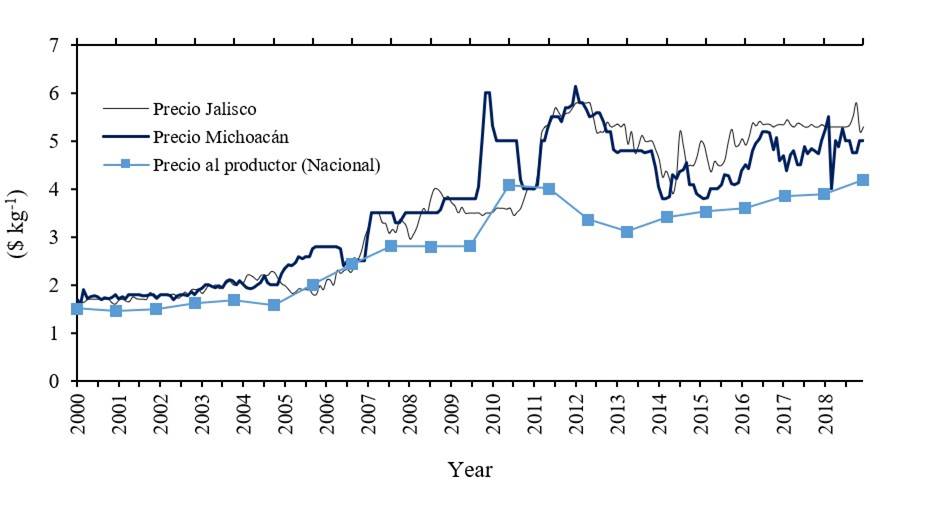
Figure 1 Graphical behavior of the price of white corn in Michoacán and Jalisco in $ kg-1. Elaboration with data from SNIIM (2018); SIAP (2020).
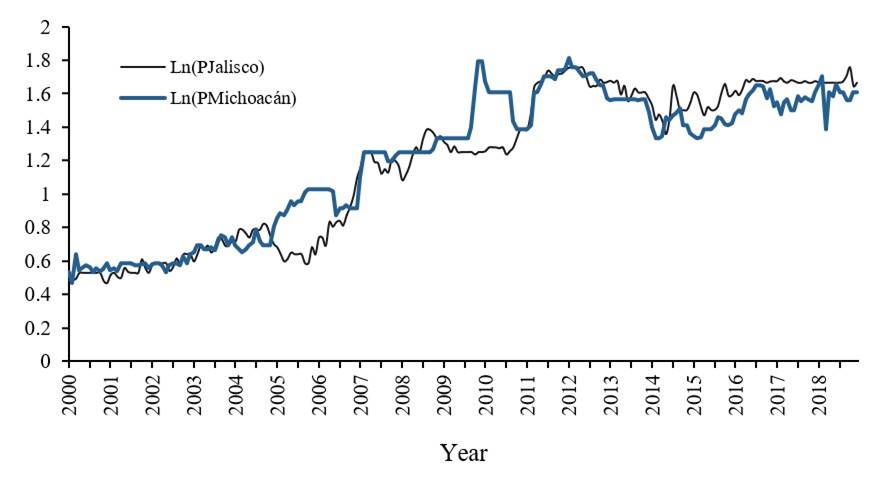
The price series transformed into logarithms also do not show constant means and variances (Figure 2). In practice, transformations can be applied to obtain stationary series, such as: simple or seasonal differentiation to eliminate the trend or induce stationarity in mean. Likewise, a Box-Cox or natural logarithm transformation can be performed to induce stationarity in variance. The first difference of the logarithm of the series was obtained to induce stationarity in mean and variance (Figure 3).

One way to check the presence of a unit root in a series is through a graphical analysis, if it presents a trend, it can be an indication that the mean and variance are not constant, an alternative to verify if the series is non-stationary is to analyze its correlogram, in a purely white noise process the autocorrelations in different lags are around zero, therefore, if the autocorrelations decrease slowly, it may indicate that the series is not stationary and, finally, some of the following tests can be applied: Augmented Dickey Fuller test (ADF) and Phillips Perron (PP) (Greene, 2012).
The series analyzed showed a slow decrease in autocorrelations; however, the unit root tests were carried out in, which the following hypothesis was tested: H0: the series have a Unit root vs H1: the series do not have a Unit root. The Augmented Dickey-Fuller (ADF) and Phillips Perron tests indicated that both series are integrated of order one I (1) in levels but are stationary by natural logarithm and first difference transformations (Table 1).
Table 1 Unit root test: Augmented Dickey Fuller and Phillips Perron.
| Variable | H0: unit root H1: no unit root | Order of integration | |
| ADF (Pr < Tau) | PP (Pr < Tau) | ||
| Michoacán | 0.7946 | 0.3146 | I (1) |
| Ln(Pmichoacán) | 0.7988 | 0.5695 | I(1) |
| ∆Ln(Pmichoacán) | <0.0001 | <0.0001 | I(0) |
| Jalisco | 0.4597 | 0.4268 | I (1) |
| Ln(Pjalisco) | 0.6396 | 0.6436 | I (1) |
| ∆Ln(Pjalisco) | 0.0002 | <0.0001 | I(0) |
*= indicates rejection of the null hypothesis at a significance level of 5%; ∆= denotes the operator of first differences and Ln denotes natural logarithm.
Autocorrelation and partial autocorrelation functions are useful in model identification; however, in ARIMA models, the model specification is subject to verification examination, diagnostic and modification (if necessary). Some tools for selecting a model are: the AIC criterion introduced by Akaike (1974) and the Bayesian information criterion (BIC) of Schwarz (1978); (Box et al., 2016).
The stage of identification of the models was carried out following the steps suggested in the methodology of Box and Jenkins, (Pankratz, 1983). Values (p, d, q) were defined considering several models by inspecting autocorrelation functions (ACF) and partial autocorrelation functions (PACF), and autoregressive AR and moving average MA parameters were estimated using ordinary least squares (Table 2).
Table 2 Estimation of ARIMA model parameters.
| Series | Adjusted model | Intercept | Estimated coefficient | log likelihood | AIC | ||
| AR (1) | MA (1) | MA (2) | |||||
| ∆Ln(PMichoacán) | AR (1) | 0.0051 | -0.0563 | 326.49 | -646.9 | ||
| Se | -0.0035 | -0.0675 | |||||
| MA (1) | 0.0051 | -0.0493 | 326.44 | -646.89 | |||
| Se | -0.0035 | -0.0636 | |||||
| ∆Ln(PJalisco) | MA (2) | 0.0054 | 0.0822 | -0.088 | 389.23 | -770.47 | |
| Se | -0.0028 | -0.067 | -0.0679 | ||||
| MA (1) | 0.0054 | 0.0816 | 388.40 | -770.8 | |||
| Se | -0.003 | -0.0737 | |||||
Se= denotes standard error.
In addition to observing the residual correlations in individual lags, it is useful to have a test that considers their magnitudes as a group (Cryer and Sik, 2008). The verification of autocorrelation in the residuals can be carried out using the statistics of Box and Pierce (1970) or Ljung-Box (1978). With the Ljung-Box test, non-autocorrelation in the residuals was verified (Makridakis et al., 1997) (Table 3), according to the p value ≥ 0.05 associated with the test, the null hypothesis was not rejected, and it was concluded that there is no autocorrelation in the errors. In the diagnostic stage of the models, it was verified that the errors have a white noise behavior and behave as a normal distribution.
Table 3 Ljung-Box test to the residuals of the ARIMA models.
| Series | Adjusted model | Ljung-Box test H0: there is no autocorrelation |
| ∆Ln(PMichoacán) | AR (1) | Q*= 20.74, df = 22, p-value= 0.5369 |
| MA (1) | Q*= 20.96, df = 22, p-value= 0.5232 | |
| ∆Ln(PJalisco) | MA (2) | Q*= 18.45, df = 21, p-value= 0.6199 |
| MA (1) | Q*= 21.139, df = 22, p-value= 0.5122 |
The constructed models were used to make point predictions outside the sample in each series. Predicted values of the data from July to December 2018 were obtained and compared with the observed data that had been reserved in the ‘validation’ set (Table 4).
Table 4 Observed and predicted prices obtained from ARIMA models in $ kg-1.
| Model | Jalisco | Michoacán | |||||
| MA (2) | MA (1) | Observed | AR (1) | MA (1) | Observed | ||
| Predicted | Predicted | Predicted | Predicted | ||||
| July 18 | 5.32874 | 5.326339 | 5.3 | 5.256702 | 5.259425 | 5 | |
| August 18 | 5.359954 | 5.354975 | 5.34 | 5.284727 | 5.286318 | 5 | |
| September 18 | 5.388794 | 5.383764 | 5.52 | 5.311693 | 5.313348 | 4.75 | |
| October 18 | 5.41779 | 5.412709 | 5.8 | 5.338864 | 5.340516 | 4.75 | |
| November 18 | 5.446941 | 5.441809 | 5.2 | 5.366171 | 5.367823 | 5 | |
| December 18 | 5.47625 | 5.471065 | 5.3 | 5.393618 | 5.39527 | 5 | |
Elaboration with data from SNIIM (2018).
Three criteria were used to measure the predictive capacity of the models: Theil’s U, the root mean square error (RMSE) and the mean absolute percentage error (MAPE) (Table 5). These have been used to evaluate prediction models in Barreras et al. (2013); Sánchez et al. (2013); Contreras et al. (2016). Theil’s U is a measure between zero and one. The Theil coefficient is expected to be equal to zero, which means that the forecast is accurate, if the Theil coefficient is equal to one, the use of the model to make predictions is not justified. In the proposed models, Theil’s U values close to zero were obtained, which indicates that the models are useful for predicting corn prices in the immediately following six months.
Table 5 Criteria of discrimination of models.
| Series | Model | Theil’s U | RMSE | MAPE |
| ∆Ln(PMichoacán) | AR (1) | 0.04176587* | 1.000933* | 8.37* |
| ∆Ln(PMichoacán) | MA (1) | 0.04192237 | 1.005392 | 8.41 |
| ∆Ln(PJalisco) | MA (2) | 0.01911703* | 0.0169519* | 2.99 |
| ∆Ln(PJalisco) | MA (1) | 0.01914904 | 0.02830746 | 2.96* |
*= model with better performance according to the criteria.
In the price series of Michoacán, the AR (1) model had the lowest mean absolute percentage error (MAPE), compared to the MA (1) model, equal to 8.37, which means that the forecast is wrong at 8.37%, in addition, this same model obtained the lowest Theil’s U equal to 0.04 and the lowest root mean square error (RMSE) equal to 1. In the price series of Jalisco, the MA (2) model performed better in two of the criteria used, compared to the MA (1) model, Theil’s U and the root mean square error with 0.01 and 0.02 respectively. The lowest mean absolute percentage error for this series was 2.96, which indicates that the forecast was wrong at 2.96%.
Currently, the price of yellow corn No. 2 of the Chicago stock exchange is taken as a reference of the price of corn in Mexico; however, Ortiz and Montiel (2017) showed, through a multivariate stochastic volatility analysis, that the market price of corn futures is not strongly related to the prices registered in some states of the country. In a comparative analysis of corn prices on the Chicago Stock Exchange and corn producer prices in Mexico, it was found that the latter are higher; however, these are different varieties (yellow and white respectively). At the same time, yellow corn prices are affected by the agricultural policy applied in the United States of America, which is characterized by maintaining high subsidies to its producers and low export prices of corn (SIAP, 2012).
Given the drawbacks of taking the price of yellow corn as an estimator of the price of white corn and given the lack of information on the future behavior of the markets, the proposed models provide a predictor of corn prices in Jalisco and Michoacán and show that these can be estimated from their own past values, however, ARIMA models have been shown to have restricted performance. Chu (1978) argues that this methodology is a simple mechanism that can be used for short-term forecasting but has a limited ability to predict unusual price movements, although, predictive power can possibly be improved by incorporating other variables.
Conclusions
The results show that Box and Jenkins’ methodology is useful for forecasting white corn prices in Michoacán and Jalisco in the short term. Corn prices in Michoacán and Jalisco can be predicted by their own past values using AR (1) and MA (2) models and these predictors constitute a useful tool in the decision-making of producers and marketers of corn-related products.
Literatura citada
Akaike, H. 1974. A new look at the statistical model identification, IEEE transactions on automatic control. 19(6):716-723. Doi:10.1109/TAC.1974.1100705. [ Links ]
Adebiyi, A.; Adewumi, O. A. and Ayo, C. K. 2014. Stock price prediction using the Arima model. UKSim-AMSS 16th International conference on computer modelling and simulation. IEEE. Reino Unido. IEEE. 2014(1):106-112. Doi: 10.1109/UKSim.2014.67. [ Links ]
Pérez-Linares, Cristina, Barreras-Serrano, Alberto, Sánchez-López, Eduardo, Figueroa-Saavedra, Fernando 2013. Uso de un modelo univariado de series de tiempo para la predicción del comportamiento de la producción de carne de cerdo en Baja California, México. México. Rev. Cien. 5(23):403-409. [ Links ]
Bowerman, B. L.; O’Connell, R. T. y Koehler, A. B. 2007. Pronósticos, series de tiempo y regresión un enfoque aplicado México. Cengage learning. 4a (Ed.). México, DF. 717 p. [ Links ]
Box, G.; Jenkins, G.; Reinsel, G. and Ljung, G. 2016. Time series analysis forecasting and control. Wiley. 5a (Ed.). New Yersey. 709 p. [ Links ]
Box, G. and Pierce, D. 1970. Distribution of residual autocorrelations in autoregressive-integrated moving average time series models. J. Am. Stat. Assoc. 65(332):1509-1526. [ Links ]
Contreras, A.; Atziry, C.; Martínez, J. L. y Sánchez, D. 2016. Análisis de series de tiempo en el pronóstico de la demanda de almacenamiento de productos perecederos. España. Estudios Gerenciales. 32(141):387-96. https://doi.org/10.1016/j.estger.2016.11.002. [ Links ]
Chu, K. 1978. Short-run forecasting of commodity prices: an application of autoregressive moving average models. International Monetary Fund. 25(1):90-111. https://doi.org/10.2307/3866657 . [ Links ]
Cryer, D. J. and Sik, K. 2008. Time series analysis with applicatios. In: Springer, R. 2a (Ed.). New York. 502 p. https://doi.org/10.1007/BF00746534. [ Links ]
Delgadillo-Ruiz, O.; Ramírez-Moreno, P. P.; Leos-Rodríguez, J. A.; Salas, J. M. y Valdez-Cepeda, R. D. 2016. Pronósticos y series de tiempo de rendimientos de granos básicos en México. México. Acta Universitaria Miltidisc. Scientif. J. 3(26):23-32. https://doi.org/10.15174/au.2016.882 . [ Links ]
Enders, W. 2015. Applied econometrics time series. Wiley. 4a (Ed.). United States of America. 498 p. [ Links ]
FIRA. 2016. fideicomisos instituidos en relación con la agricultura. Panorama agroalimentario 2016. [ Links ]
FIRA. 2019. fideicomisos instituidos en relación con la agricultura. Panorama agroalimentario 2019. [ Links ]
Gujarati, D. N. and Porter, D. C. 2010. Econometría. McGraw-Hill Publishing Educacion. 5a (Ed.). México. 946 p. [ Links ]
Greene, W. H. 2012. Econometric analysis. Pearson. 7a (Ed.). New York University. 1241 p. [ Links ]
Jamal, F.; Ezzine, L. and Aman, Z.; El Moussami, H. and Lachhab, A. 2018. Forecasting of demand using ARIMA model. Inter. J. Eng. Bus. Manag. 10(1):1-9. Doi: 10.1177/18479790 18808673. [ Links ]
Ljung, G. and Box, G. 1978. On a measure of a lack of fit in time series models. Biometrika. 65(2):297-303. Doi:10.1093/biomet/65.2.297. [ Links ]
Luis-Rojas, S.; García-Sánchez, R.; García-Mata, R.; Arana-Coronado, O. A. and Gonzáles-Estrada, A. 2019. Metodología Box-Jenkins para pronosticar los precios de huevo blanco pagados al productor en México. Agrociencia. 6(53):911-925. [ Links ]
Makridakis, S.; Wheelwright, S. C. and Hyndman, R. J. 1997. Forecasting, methods and applications. Jhon Wiley and Sons. 3a (Ed). EU. 656 p. [ Links ]
Marroquín, G. y Chalita, L. E. 2010. Aplicación de la metodología Box-Jenkins para pronóstico de precios en jitomate. México. Rev. Mex. Cienc. Agríc. 4(2):573-577. http://www.redalyc.org/articulo.oa?id=263119723008. [ Links ]
Ortiz A.y, MontielA. N. 2017. Transmisión de precios futuros de maíz del chicago board of trade al mercado spot mexicano. México. Contaduría y Administración. (62):924-940. https://doi.org/10.1016/j.cya.2016.01.004. [ Links ]
Pankratz, A. 1983. Forecasting with univariate Box-Jenkins models concepts and cases. Jhon Wiley and Sons. EU. 588 p. [ Links ]
Quintana, L. y Mendoza, M. A. 2010. Econometría aplicada utilizando R. Universidad Nacional Autónoma de México (UNAM). México. 358 p. [ Links ]
SAGARPA. 2017. Secretaría de Agricultura Ganadería Desarrollo Rural Pesca y Alimentación. Planeación agrícola nacional 2017-2030. México, DF. [ Links ]
Sánchez- López, E.; Barreras-Serrano, A.; Pérez-Linares, C.; Figueroa-Saavedra, F. y Olivas-Valdez J. A. 2013. Aplicación de un modelo ARIMA para pronosticar la producción de leche de bovino en baja california, México. Trop. Subtrop. Agroecosys. 3(16):315-324. [ Links ]
SIAP. 2020. Servicio de Información Agroalimentaria y Pesquera. https://nube.siap.gob.mx/ cierreagricola/. [ Links ]
SIAP. 2019. Servicio de Información Agroalimentaria y Pesquera . Panorama agroalimentario 2019 . México, DF. [ Links ]
SIAP. 2012. Servicio de Información Agroalimentaria y Pesquera . Situación actual y perspectivas del maíz en México 1996-2012. http://www.campomexicano.gob.mx/portal-siap/Integracion/EstadisticaDerivada/ComercioExterior/Estudios/Perspectivas/maiz96-12.pdf. [ Links ]
SNIIM. 2018. Sistema Nacional de Información e Integración de Mercados. Secretaría de Economía. http://www.economia-sniim.gob.mx/nuevo/. [ Links ]
Schwarz, G. 1978. Estimating the dimension of a model. Annals of statistics. 6(2):461-464. MR 468014. doi:10.1214/aos/1176344136. [ Links ]
Received: January 01, 2022; Accepted: March 01, 2022
 Este es un artículo publicado en acceso abierto bajo una licencia Creative Commons
