


Services on Demand
Journal
Article
 text in
  English (pdf)
 Article in xml format
 Article references
 Send this article by e-mail
Indicators
-
 Cited by SciELO
 -
 Access statistics
Related links
-
 Similars in
SciELO
Similars in
SciELO
Share

 Permalink
Revista mexicana de ciencias agrícolas
Print version ISSN 2007-0934
Rev. Mex. Cienc. Agríc vol.7 n.7 Texcoco Sep./Nov. 2016
Articles
Sample sizes that ensuring accuracy to estimate prevalence of plants under inverse sampling
1 Universidad de Colima-Facultad de Telemática. Bernal Díaz del Castillo Núm. 340, Villas San Sebastián, 28045. Colima, México. (oamontes2@hotmail.com; mandrad@ ucol.mx).
The detection of a rare or scarce event (with low prevalence ≤ 0.1) in the design of agricultural experiments of a population consumes many resources. Therefore, one resorts to the inverse sampling (negative binomial) which consists of a series of tests with binary response (presence or absence) in which not stop sampling until a predetermined individuals with the trait of interest number. Therefore a method is proposed to calculate the required sample size (number of positive units) under inverse sampling ensures accurate estimated proportion because it ensures that the amplitude (W) of the confidence interval (IC) will be equal to, or more narrower than, the desired amplitude (ω), with a probability y (assurance level). Given the complex and laborious process of estimating both the sample size and parameters of interest (proportion, variance, standard deviation, total and confidence intervals for the proportion and total) free software is proposed for inverse sampling under the approach of accuracy in the estimation of parameters that automates the calculation of sample sizes and parameters of interest. In addition, the software provides a graphical, easy, safe and user friendly interface. The using the formula proposed for ensuring a probability y (assurance level > 0.5) fixed a priori accuracy is met IC is recommended. Which produces more accurate study performed interest.
Keywords: confidence interval; low prevalence; parameter estimation
La detección de un evento raro o escaso (con prevalencia baja p ≤0.1) en el diseño de experimentos agrícolas de una población consume muchos recursos. Por ello, se recurre al muestreo inverso (binomial negativo) el cual consta de una serie de ensayos con respuesta binaria (presencia o ausencia) en el que no se deja de muestrear hasta obtener un número predeterminado de individuos con la característica de interés. Por ello se propone un método para calcular el tamaño de muestra requerido (número de unidades positivas) bajo muestreo inverso que asegura exactitud en la proporción estimada porque garantiza que la amplitud (W) del intervalo de confianza (IC) será igual a, o más estrecha que, la amplitud deseada (ω), con una probabilidad γ (nivel de aseguramiento). Dado lo complejo y laborioso del proceso de estimación tanto del tamaño de muestra y de los parámetros de interés (proporción, varianza, desviación estándar, total e intervalos de confianza para la proporción y el total) se propone un software de distribución libre para muestreo inverso bajo el enfoque de exactitud en la estimación de parámetros que automatiza el cálculo de tamaños de muestra y de los parámetros de interés. Además el software provee una interfaz gráfica, fácil, segura y amigable con el usuario. Se recomienda el uso de la fórmula propuesta pues garantiza que con una probabilidad γ (nivel de aseguramiento ≥0.5) la precisión fijada a priori del IC se cumpla. Lo cual produce mayor exactitud en el estudio de interés realizado.
Palabras clave: estimación de parámetros; intervalo de confianza; prevalencia baja.
Introduction
To ensure transparency of plant health is necessary to control the spread of ensuring the health of plants in a given population diseases. Improved plant health has clear health of man (phytopathological disease control, food safety, innocuousness and food sanitation), positive implications for economic development and agricultural production benefits. That is why the developed and developing country have given much importance to monitoring programs and monitoring of plant systems (Ragan, 2002).
Within a population there are elements with low prevalence rates (a small subset of the total population), these are called rare, rare or elusive (Graham and Dallas, 1988; Sudman et al, 1988) are as typical cases plants, animals and people with diseases, clinical treatments, and in general all those groups with low frequency units having a particular characteristic. Some authors like Czaja et al. (1996) find that rare populations are present in less than 3% of the universe of study.
To estimate the prevalence plant (absence of disease in populations) sampling methods are paramount (Hernández-Suárez et al., 2008). For this reason, the calculation of the optimal sample size is important in the design of agricultural experiments for estimating proportions populations, including the prevalence of disease (Fosgate, 2007).
In the estimation of parameters associated with few characteristics of a population, the traditional sample designs do not offer the best methodological conditions, mainly because of the difficulty of locating items with the desired characteristic. That is why that should be used for other special occasions, such as the inverse or negative binomial sampling techniques. This method has been used in the field of hematology, genetics, inspection (Zhu and Lakkis, 2014), epidemiological investigations (Singh and Aggarwal, 1991; Lui, 2001; Tang et al, 2008), ecology (Sheaffer and Leavenworth, 1976; Krebs, 2001), detection of diseases in plants and animals (Madden et al. 1996), measuring the effectiveness of clinical treatments (George and Elston, 1993) among others.
To detect the presence of a rare event in a population is required to try a sufficiently large number of individuals, and the cost of such tests usually exceeds human and financial resources available. Besides being a laborious activity, consuming time and effort. The inverse sampling is an ancient method (George and Elston, 1993) for estimating a proportion p, it is based on the negative binomial distribution with a series of trials Bernoulli where it is not left to sample until a desired number of individuals with characteristic of interest. However, when the probability of finding the desired attribute is practically nil (≤ 0.1), using the binomial sampling (where the number of elements in the sample is preset) is not the best option because according Haldane (1945) use a binomial distribution does not always provide an unbiased and accurate estimate of p when it is small (p ≤ 0.1).
George and Elston (1993) recommend the use of geometric sampling (consisting stop the sampling process until it is an individual with the characteristic of interest) when the probability of the event of interest is small. In his research obtaining confidence intervals (IC's) for prevalence based on individual tests and under a geometric model is provided. Also, Haldane (1945) asserts that the use of a binomial distribution does not always provide an unbiased and accurate estimate of p when it is small (p ≤ 0.1). Lui (2000) extended the work of George and Elston (1993) for IC's to consider using negative binomial sampling (stop the sampling process until r > 1 individuals with the characteristic of interest are) and showed that as r increases, the amplitude of the confidence interval (IC) is reduced. This extension applies to individual tests.
Historically, researchers have emphasized planning sample size in empirical research, to obtain useful information from experimental and observational studies from a perspective of pure analytical power. Although the structure of analytical power has dominated the way researchers conceptualize planning sample size, is neither the only, nor the best approach that can be taken to estimate the appropriate number of participants to be included in any study of interest. Often estimating exact parameters is potentially even more significant goal the obtaining statistical significance (Kelley et al, 2003). This shows that the appropriate method for planning the sample size, and the appropriate size of the sample itself, depend on the desired goals in an investigation.
An alternative approach by Kelley (2007) for the frame of analytical power for determining sample sizes is ensuring the accuracy in estimating parameters (AIPE). The aim of AIPE is to ensure that the estimated parameters correspond to the accuracy set to estimate that the population parameter. Authors like Montesinos-López et al. (2011) have developed procedures for calculating sample sizes under the AIPE approach, an approach that guarantees short IC's for estimating parameters under binomial sampling and testing group. The IC's also transmit information to accurately determine the magnitude of the effect from the available data (Beal, 1989; Montesinos-López et al, 2012). Therefore, the determination of sample sizes under this approach can contribute to infer stronger and precise theories about a phenomenon under study.
Perform the necessary calculations to determine sample sizes and estimate other important parameters under reverse sampling is undoubtedly a laborious task. Montesinos-López et al. (2012) propose a computational algorithm in the R statistical package where sample sizes are calculated focusing AIPE for reverse sampling, but it is noteworthy that only focuses on the sampling groups (Group Testing), besides lacking a graphics, friendly and easy user interface.
Therefore, the purposes of this article are: 1) to derive an expression for calculating sample sizes for estimating a proportion (p) under inverse sampling (negative binomial) under the AIPE approach, 2) show through examples calculation process for sample size and 3) develop software for the determination of sample sizes and the estimation of parameters of interest under this approach.
Materials and methods
Suppose Yi= yi individuals are tested to find the first positive individual and Y1, Y2, Y3,...Yr are observed for the r-th positive individual. Since, Yi (i= 1, 2,.. .,r) has a geometric distribution. Therefore, the total number of individuals is recorded to find positive individuals r is equal to  . The prevalence is denoted by p, the number of tested to find the first positive individuals individual is Yi= yi, and the number of times the experiment is carried out is denoted by r. It is important to note that this document is considered that: (i) the sample size is the value of r representing the required number of positive individuals to stop the process of sampling and testing, and (ii) the total number of individuals tested is the value of . Therefore, sufficient and complete statistic has a negative binomial distribution (dbn) with r parameter and probability of success p (George and Elston, 1993). According to George and Elston (1993) maximum likelihood estimation (EMV) of p using inverse sampling is:
 1)
1)
Where: r is the required number of fixed positive individuals. This EMV of p for reverse sampling assumes a perfect diagnostic test (specificity and sensitivity equal to one). Moreover, the variance of p according to George and Elston (1993) is it given by 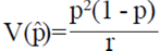 taking into account the correction factor of finite population is equal to
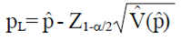
  where q= (1 - p). According to George and Elston (1993) the IC of Wald is:
 2)
2)
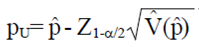
Where: Z1-α/2 is the quantile 1-α/2 standard normal distribution, and p is the EMV. This approach IC is easy to calculate and derive formulas allows the size of the sample so closed. However, when r is small, the normal approach to EMV is doubtful; since in such cases the IC of Wald often produces negative endpoints. Furthermore, the probability of coverage of IC's constructed by IC of Wald is often less than 100 (1 - α)%.
The amount  (added and subtracted from the observed ratio, p) in Ec. 2 is defined as W/2 (where W is the width of IC; W o W/2 can be set a priori by the researcher depending on the desired accuracy). The IC amplitude observed for any embodiment of this confidence interval (From Ec. 2) can be expressed as:
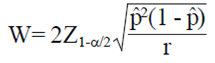 3)
3)
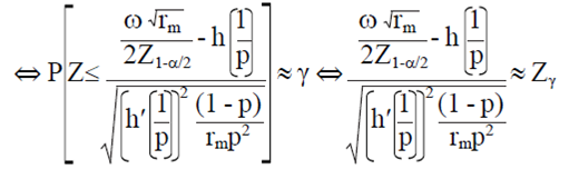
Be the desired amplitude ω IC; then the AIPE approach basically find the minimum sample size that ensures that the expected amplitude of the IC is sufficiently narrow (Kelley, 2007; Kelley and Rausch, 2011). In other words, the approach seeks AIPE minimum sample size such that E (W) ≤ω. The problem is that the expected amplitude of the IC is an unknown quantity, but can be approximated.
Therefore, the expected value of W is:  (Lui, 1995).
Now if the E (W) is set to the desired amplitude of the IC, ω
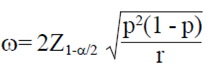 4)
4)
According to Lui (2001) by solving r (Ec. 4) the following formula is obtained:
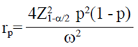 5)
5)
However, Ec. 5 requires the population value of p, which is known in practice and is replaced by an estimate of the actual ratio. Although Ec. 5the sample size necessary to achieve the desired amplitude of the IC, E(W), which is close enough to the estimated proportion is provided. However, this does not guarantee that any particular IC, the expected amplitude of the observed IC, E(W), is sufficiently narrow, because the expected value only approximates the average interval width confidence. Kelley and Rausch (2011) argue that this problem is similar to the case where an average is estimated from a normal distribution, although the sample mean is an unbiased estimator of the population mean, it is almost certain that the sample mean is smaller or larger than the value of the population. This is because the sample mean is a continuous random variable, as is the width of the IC, because both are based on random data. Therefore, about half of the time width calculated IC is greater than the previously especified width (Kelley and Rausch, 2011).
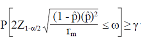
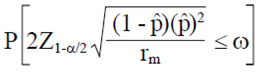
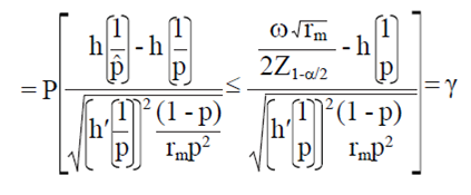
Because Ec. 3 uses an estimate of p, the width of the IC (W) is a random variable fluctuate from sample to sample. This implies that rp using Ec. 5, about 50% of the sampling distribution of W is less than © (third column of Table 1). To demonstrate this, you calculate the probability of an amplitude of less IC to the specified value (ω). This can be calculated by:
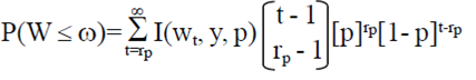
Where: I (wt, y, p) is an indicator function that shows whether the actual IC width calculated using Ec. 3 es ≤ ω, p is the true proportion of the population and rp is the size of the sample obtained. Ec. 5. Due to computational limitations the following approximation to calculate this probability is used.
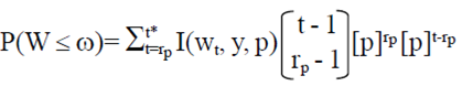 6)
6)
Where:t= rp, rp + 1, rp+2,...t*, and W is considered a random variable since the exact value p is not known t* is the value that satisfies P(T ≤ t*)= 0.9999. The value of t* it is used as the operation in the R package may not add up to infinity.
Derivation low sample size AIPE for reverse sampling
The procedure for deriving the expression for calculating sample size for estimation of a ratio (p) for sampling under AIPE reverse approach is shown.
Suppose Yb.. .,Yr is a random sample of size r of a geometric distribution (p). Let  with
with 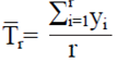 .
.
Then for 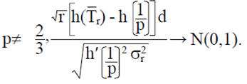
That is, 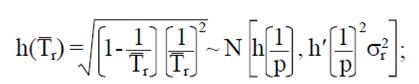 where
where 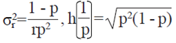 and
and 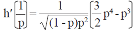 .
.
Note that T  Then if
  ,
,  is differentiable with respect to a
 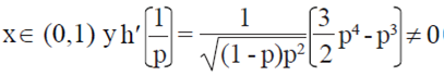 . For p
  , then using the delta method (Oehlert, 1992) is obtained,
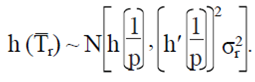
Then, the smallest integer value rm such that:
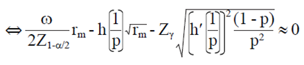
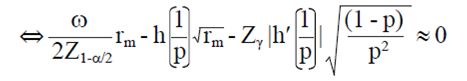 7)
7)
Note that Eq. 7 has a quadratic form ax2 + bx + c= 0, with 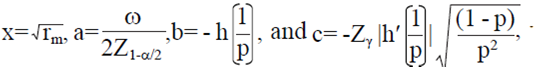 with two solutions given by
  . Taking
  Therefore, for a fixed ©, the rm desired is given by
  where after replacing
  and
and  is obtained
  7)
7)  . 8)
. 8)
This procedure shows the expression for calculating sample sizes ensuring accuracy in the estimation of parameters of interest.
Results and discussions
Understatement sample size using Ec. 5.
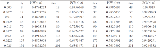
To show the extent to which rp is underestimated by Ec. 5, an example (Table 1) in which Ec. 6 is used is provided to calculate P (W ≤ ω) i.e., the probability that W is less than or equal to the desired amplitude (co) for IC a given rp (number positive units) obtained with Ec. 5. The numerical value example in Table 1 is given for various values of the population proportion (p) with IC at 95%, and a desired width ω = 0.007. In the Table 1 presents the preliminary sample size rp calculating Ec 5, and three other increases: rm10= rp + 10, rm20= rp + 20 and rm40= rp + 40. For each sample size, the probability that W is less than the specified value (ω = 0.007) is P (W ≤ ω) and is calculated using Ec. 6. This is done to show that the required number of positive units to estimate the proportion (rp of the second column) calculated using Ec. 5 has a probability of about 0.50 that W ≤ ω =0.007 (third column). For example, when p= 0.02, the preliminary sample size (rp ) is 48 and the probability of obtaining a W ≤ ω = 0.007 is 0.4738842. With p = 0.02, rp= 123, can only be 49.12% sure that W will ≤ ω = 0.007. When the number of positive units increases by 10 (rm10 , fourth column) or 20 (rm20, sixth column), the probability P (W ≤ ω = 0.007) increases.
For example, when p= 0.0125, there rm20= 68 units in the sample with P (W ≤ ω = 0.007)= 0.9114708; for rm40= 88 positive units in the sample, P (W ≤ ω =0.007)= 0.9962598. Therefore, the results in Table 1 show that a sample size (number of positive units) is required to ensure high P (W ≤ ω = 0.007), greater than the value rp calculated Eq. 5. Furthermore, Table 1 shows that in the 9 cases the size of the resulting preliminary sample (number of positive observations) using Ec. 5 produces at P (W ≤ ω) < 0.50, that is, 100% of the time P (W ≤ ω = 0.007) is less than 50%.
For estimation of plant prevalence low inverse sampling
As an example of estimation for the use of the techniques mentioned develops the following case:
Example 1. Suppose a researcher is interested in estimating the proportion of virus infected plants in an agricultural company, with a population of N= 4 300 plants, it is decided to use low single inverse sampling random sampling (MAS). Since the prevalence of infected plants is set low to stop the sampling process until they are r= 5 infected plants. In addition, the registration of all plants is carried extracted and analyzed. It is, without replacement plant extract and analyze if you are infected. This extraction process will continue until 5 are infected plants. The total number of analyzed to find the five plants was infected n= 250. The calculations are made with an accuracy of10% (d= 10/100) of the preliminary ratio (p), reliability (1 - a) of 95% (a= 95/100) and a level of assurance (γ) of 99% (γ = 99/100). In the Table 2 shows the calculations for estimating several parameters of interest are shown.
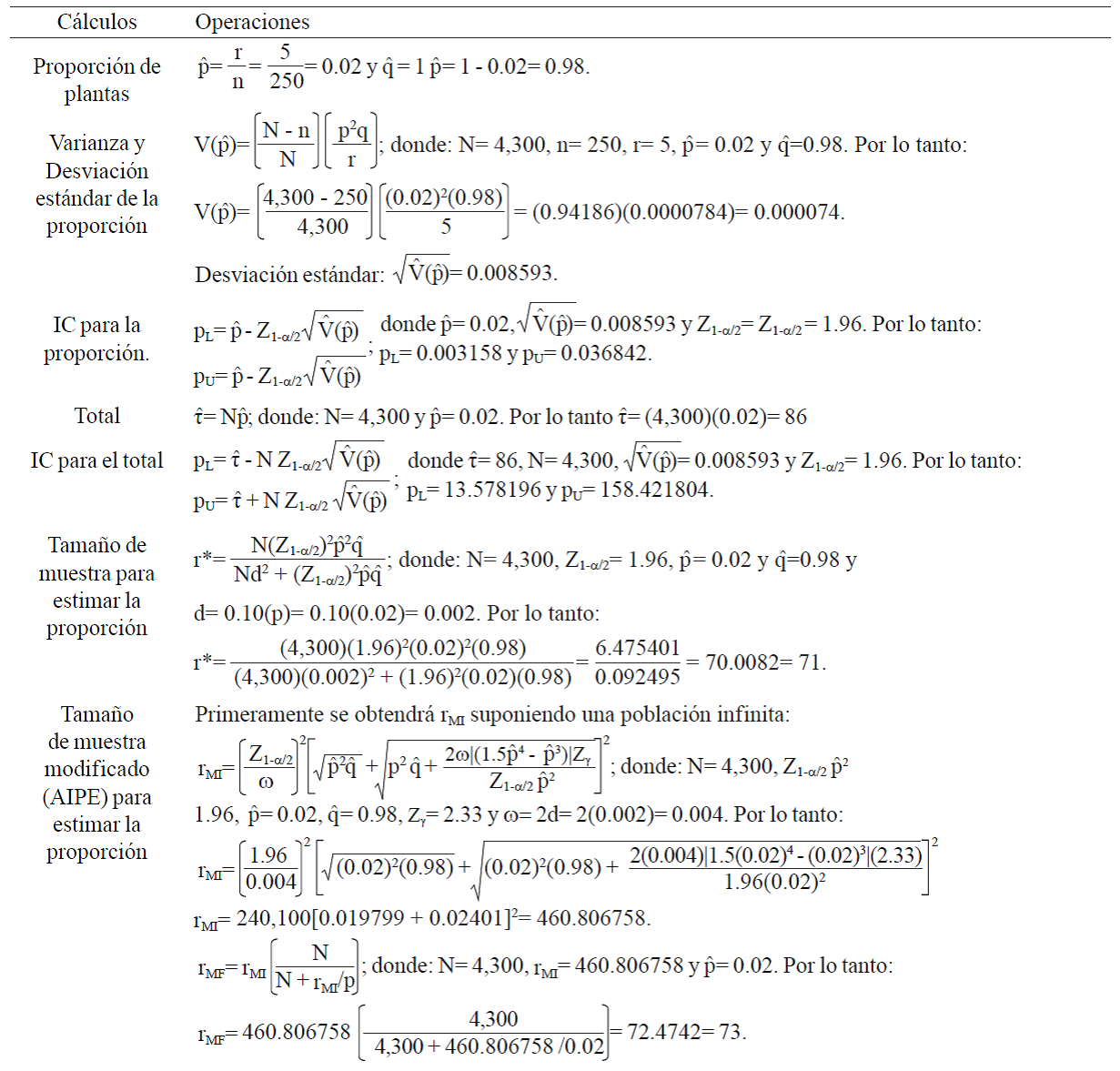
Table 2 is that the proportion of infected plants is p= 0.02 with 95% reliability is estimated that the real ratio is 0.036842 and 0.003158, i.e. between 0.31 to 3.68%. It is estimated that the actual total is 86 infected plants, and between 13.57 and 158.42 is. Finally you have to sample sizes under the traditional approach, and under the AIPE approach are 71 and 73 respectively.
Clearly manually do the calculations in Table 2 I is slow, laborious and with a high probability of being wrong. Therefore, the need to develop a free software that allows obtaining these parameters quickly, effectively and safely considered.
Software for example reverse-sampling
The software sampling was raised from two purposes: a) to determine the sample size for a study under the scheme of inverse sampling ratio and b) the estimation of the parameters resulting from applying this sampling scheme.
To calculate a sample size there is a contradiction in having to meet in the design phase, the value of a parameter that can only be estimated once extracted from the sample. To solve this problem you have two options, the first is to estimate the parameter from a pilot sample; the second is to obtain an acceptable value through the references have jobs or similar experiences already made. In the software for reverse sampling was chosen option 1. In addition, it is also required to specify the level of significance (a) which is usually less value than 0.2 (20%) and accuracy, which is defined as estrangement maximum time allowed between the parameter and its estimate. The software allows the user to provide the required accuracy (directly) or obtained indirectly as a percentage of the estimated proportion preliminary.
However, since the sample sizes are calculated under the AIPE approach must also specify the level of assurance (γ) and this should be a value greater than 0.5 (50%).
Then using the software is illustrated by solving Example 1. First the data requested by the software are introduced and click on calculate as illustrated in Figure 1.
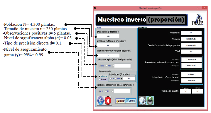
We should not lose sight that the sample of 250 is a pilot shows that only serves to obtain the final sample. In this case can be seen in the results area (Figure 1) modified size sample (final), it is 73 plants. This sample size ensures that the accuracy will be fulfilled with a certainty of 99%.
Importantly, this sample size is greater than the estimated sample size traditionally is 71 (Figure 1), which only ensures that the required accuracy, 50% of the time is met, because does not take into that the preliminary estimated sample parameter is an estimate. Therefore, it is clear that the sample size under the AIPE approach (modified sample size) is usually greater to ensure the specified level of assurance.
Finally the researcher will estimates of the parameters of interest (percentages, totals, IC's) with the final sample using the same software but using the information collected from the final sample. That is, the preliminary sample is used only to obtain the final sample and to verify possible problems in the implementation of the survey. Therefore, the researcher must conduct the survey again but stop the sampling process until you find 73 (size modified sample) positive elements and the information gathered can use the same software for estimating parameters of interest which shall be valid estimates for the entire study population.
It is noteworthy that the software is not limited to the inverse sampling, but can also be used for sampling: simple, systematic, random stratified random, cluster at one stage, to estimate an average or proportion and even with methods such as randomized response (Horvitz version) and test group (group testing). You can consult the detailed manual log of all software capabilities in https://dl.dropboxusercontent.com/u/97440566/manual%20tmapep.pdf.
Conclusions
The formula presented for the calculation of sample size to estimate the prevalence of plants under reverse AIPE sampling approach ensures that with a probability y (assurance level ≥ 0.5) fixed a priori accuracy of the IC is met. Which produces more accurate study performed interest.
The free distribution of software designed to reverse sampling is an excellent tool that enables researchers and students to achieve accurate estimates on the parameters of interest and is recommended when the ratio estimate is rare. While presenting the cases shown is limited, since only an example for the scheme inverse sampling is provided, this software can be used for on time or interval estimate an average, a proportion or a total under simple random sampling, stratified, systematic cluster and a stage and even for highly specialized sampling schemes such as reverse sampling and testing randomized response group. Although only one type of use of the software is illustrated clearly is used both for determining the sample size and for estimating parameters of interest using a pilot sample. Although the software requires the user to consider a pilot sample, and determine the final sample size, this ensures quality in the final estimates.
For the researcher or student succeeds in using the software fully, not only to reverse sampling should understand what this sampling scheme and its characteristics, as well as having clear parameters to estimate for the corresponding study. Therefore, if all decisions at this stage are justified properly, the software developed will be of great help, because, from the point of view statistical and computational software is very reliable.
Literatura citada
Beal, S. L. 1989. Sample size determination for confidence intervals on the population mean and on the difference between two population means. Biometrics. 45:969-977. [ Links ]
Czaja, R.; Snowden, C. B. and Casady, R. 1996. Reporting vias and sampling errors in a survey of a rare population using multiplicity counting rules. Journal of the American Statistical Association. 81(394):411-419. [ Links ]
Fosgate, G. T. 2007. A cluster-adjusted sample size algorithm for proportions was developed using a beta-binomial model. Journal of clinical epidemiology. 60(3):250-255. [ Links ]
George, V. T. and Elston, R. C. 1993. Confidence limits based on the first occurrence of an event. Statistics in Medicine. 12(7):685-690. [ Links ]
Graham, K. and Dallas, A. 1988. Sampling rare populations. J. Royal Statistical Soc. 149:65-82. [ Links ]
Haldane, J. B. 1945. On a method of estimating frequencies. Biometrika. 33(3):222-225. [ Links ]
Hernández-Suárez, C. M.; Montesinos-López, O. A.; McLaren, G. and Crossa J. 2008. Probability models for detecting transgenic plants. Seed Sci. Res. 18(02):77-89. [ Links ]
Kelley, K. 2007. Sample size planning for the coefficient of variation from the accuracy in parameter estimation approach. Behavior Research Methods. 39(4):755-766. [ Links ]
Kelley, K.; Maxwell, S. E. and Rausch, J. R. 2003. Obtaining power or obtaining precision: delineating methods of sample-size planning. Evaluation & the health professions. 26(3):258-287. [ Links ]
Kelly, K. and Rausch, J. R. 2011. Sample size planning for longitudinal models: Accuracy in parameter estimation for polynomial change parameters. Psychological Methods. 16(4):391-405. [ Links ]
Krebs, C. J. 2001. Ecology. The experimental analysis of distributions and abundance. Harper and Row publishers. Michigan, USA. 801 p. [ Links ]
Lui, K. J. 2001. Estimation of rate ratio and relative difference in matched-pairs under inverse sampling. Environmetrics. 12(6):539-546. [ Links ]
Madden, L. V.; Hughes, G. and Munkvold, G. P. 1996. Plant disease incidence: inverse sampling, sequential sampling, and confidence intervals when observed mean incidence is zero. Elsevier. 15(7):621-632. [ Links ]
Montesinos, L. O. A.; Montesinos, L. A.; Crossa, J. and Kent, E. 2012. Sample size under inverse negative binomial group testing for accuracy in parameter estimation. Plos One. 7(3):1-10. [ Links ]
Montesinos, L. O. A.; Montesinos, L. A.; Crossa, J.; Eskridge, K. and Sáenz, C. R. A. 2011. Optimal sample size for estimating the proportion of transgenic plants using the Dorfman model with a random confidence interval. Seed Sci. Res. 21(3):235-246. [ Links ]
Oehlert, G. W. 1992. A note on the delta method. The American Statistician. 46(1):27-29. [ Links ]
Ragan, V. E. 2002. The animal and plant health inspection service (APHIS) brucellosis eradication program in the United States. Veterinary Microbiol. 90(1):11-18. [ Links ]
Sheaffer, R. L. and Leavenworth, R. S. 1976. The negative binomial model for counts in units of varying size. J. Quality Technol. 8(3):158-163. [ Links ]
Singh, P. and Aggarwal, A. R. 1991. Inverse sampling in case control studies. Environmetrics. 2(3):293-299. [ Links ]
Sudman, S.; Sirken, M. and Cowan C. 1988. Sampling rare and elusive populations. Science. 240(4855):991-996. [ Links ]
Tang, M. L.; Liao, Y. J. and Ng, H. K. T. 2008. On test of rate ratio under standard inverse sampling. Computer methods and programs in biomedicine 89(3):261-268. [ Links ]
Zhu, H. and Lakkis, H. 2014. Sample size calculation for comparing two negative binomial rates. Statistics in Medicine. 33(3):376-387. [ Links ]
Received: February 2016; Accepted: May 2016
 Este es un artículo publicado en acceso abierto bajo una licencia Creative Commons
