Introduction

The distribution of fresh guava in Mexico, has been given as an important part in the consumption of each person since guava is one of the fruits with highest vitamin content (highlights its high content of vitamin C) and digestive properties (high digestibility coefficient and high fiber content). In 2013 there were more than 290 thousand tons, its distribution nationwide must be fair in order to have a per capita consumption in each state. Therefore, through modeling equable distribution in the population using logistics, it could supply fresh guava to Mexican population.

According to ^{Ballou (2004)}, the most important product characteristics that influence logistics strategy are the attributes of the product itself, life cycle, weight, volume, value, if they are perishable or not, flammability and substitutability . When viewed in various combinations, these characteristics are an indication of storage requirements, inventories, transportation, materials handling and order processing. These attributes can be discussed better if grouped into five categories: life cycle, weight-volume ratio, value-weight ratio and substitutability and risk characteristics. Transportation generally represents the single most important element in logistics costs for most businesses. It has been observed that freight movement absorbs between one and two thirds of total logistics costs.

Considering that guava is a highly perishable fruit and marketing of fresh produce, so far lacks adequate infrastructure, it is reasonable to think that marketing prospects perhaps should aim towards transformation, it should be noted at this point the technological versatility of guava as raw material, and the high nutritional content of their products, showing salient advantages that allow better accessibility of the product to a larger part of the population, which in these times is losing the habit of fresh consumption and being replaced by processed products. Seasonality of guava production has generated that this fruit is present in the market for only certain times of the year; but if considered for industrialization or transformation, market presence (and consequently in the mind of the consumer), may increase significantly, which will increase the placement of the fruit in the general population, increased consumption per capita.

Of course, to produce and market this type of food is necessary to use and generate knowledge and new technologies. It also requires a different organization for its transportation, storage, processing and marketing of these differentiated, functional, ethnic and individual foods, are forming networks of value. Consumption in Mexico, it is present given the knowledge of the nutritional properties of guava, but because only in the central region is produced effectively, requires distribution to other states that are still in deficit consumption or its small production is not optimal for their own consumption.

Materials and methods

In this study only seven producing states are contemplated as logistics region: Aguascalientes, Guerrero, Jalisco, State of Mexico, Michoacán, Querétaro and Zacatecas; states that are mostly profitable in fresh guava production, allowing to supply the domestic and international markets, because it has enough farmland and techniques to substantially increase productivity given its precocity and high nutrient content (Plan Rector del Sistema Producto Guayaba, 2008).

The methodology used to perform this study includes:

The model to develop is in a closed market, where only considers domestic production and consumption. For model formulation it requires knowledge of the decision variables as objective function and supply and demand constraints. To define the objective function must meet all transportation costs for each of the origins to each of the destinations. In supply constraints, the origins and amounts available and in demand, destinations and quantities demanded.

For the transportation model, information sources were obtained from statistical sources and databases consulted in the Agrifood and Fisheries Information of the Secretariat of Agriculture, Livestock, Fisheries and Food (SAGARPA SIAP, 2010) from which was obtained guava production per state and per cycle, thus plantings; the National Population Council (CONAPO) and the population and housing census 2010 from INEGI (official information) and transportation costs from the supplying centers to demanding markets obtained the formulation:

Where: CTRANS= transport cost; CF= fixed costs: wages and salaries of corporate and management, insurance, taxes, duties and domestic services; CV= variable costs: fuel, maintenance, tires, truck expenses, operator; D= distance.

In addition to these, factors such as engine performance, diesel cost and depreciation were added directly. The transportation problem can be fitted to a mathematical model and the number of variables is less than 500, so it was decided to use programming package LINDO 6.1 for best results. In the transportation model for closed market it was considered only domestic production and consumption. It sought to optimally distribute the fruit from those entities with surplus production. For the solution to the closed market model, once identified the origins, the amount offered, destinations for demanded guava and transportation costs per ton was formulated the closed market model. In the case of open market it will only record data from external demands, thus as costs to transport the product.

In developing the objective function are considered transportation costs C_ij from origins (n) to each destinations (m) multiplied by amount (X) that should be sent to each of them and is represented with X_nm. The objective function of the model is as follows:

Where: Z₀= value of the objective function; i= index from state of origin (supplier), where i= 1,2, ..., m, j= index from destination state (demand), where j= 1,2, ..., n; X_ij= decision variable that is determined with the solution model is the amount of allocated guava from origin i to destination j; C_Ij= coefficient from Xij variable, represents the amount with which each unit from Xij variable contributes, to the desired total value in the objective. The model represents the transportation cost per ton from origin i to destination j.

Each model has many supply constraints as the number of origins i that exist and so many demand constraints as the number of destinations j. Abstractly closed market models, are as follows:

Subject to:

A surplus model

In the closed market transportation model it was considered only domestic production and domestic consumption. It sought to optimally distribute the fruit from those entities with surplus production towards deficit states.

By solving the model the value of the objective function is obtained and which will be the optimal quantities to be sent from each origin to each destination. The origins that in the models do not distribute the total of its surplus production; i.e. that are left with values in the reduced cost will be considered as the least located origins, indicating the cost or decrease that the objective function will have per each unit that is intended to add to its realization. And the origins remaining with zero value in the reduced cost are considered as the best-located origins. Also in the model output the results of minimal cost indicate how much the objective function would increase if one more unit of supply was added in the best located places.

Results and discussion

When obtaining state information of fresh guava production for marketing and population by state; proceed to obtain the surplus and deficit states according to state consumption and per capita consumption, being as follows (Table 1).

Table 1. Production, consumption and availability of fresh guava by state, 2010. 

Estado	Producción oferta (t)	Población	Consumo total (t)	Disponible (t)
Aguascalientes	72 459.19	1 184 996	72 459.19	70 099
Baja California	4	3 155 070	4	- 6 280.02
Baja California Sur	33.25	637 026	33.25	- 1 235.53
Campeche	0	822 441	0	- 1 638.07
Coahuila de Zaragoza	0	2 748 391	0	- 5 474.03
Colima	399.06	650 555	399.06	- 896.66
Chiapas	418.2	4 796 580	418.2	- 9 135.25
Chihuahua	0	3 406 465	0	- 6 784.73
Distrito Federal	0	8 851 080	0	- 17 628.89
Durango	478.73	1 632 934	478.73	- 2 773.62
Guanajuato	581.2	5 486 372	581.2	- 10 346.12
Guerrero	2 068.55	3 388 768	2 068.55	- 4 680.94
Hidalgo	372	2 665 018	372	- 4 935.97
Jalisco	2 000.87	7 350 682	2 000.87	- 12 639.64
México	1 075.7	15 175 862	1 075.7	- 29 150.39
Michoacán de Ocampo	113 760.14	4 351 037	113 760.14	105 094.08
Morelos	158.47	1 777 227	158.47	- 3 381.27
Nayarit	787.72	1 084 979	787.72	- 1 373.26
Nuevo León	0	4 653 458	0	- 9 268.39
Oaxaca	54.1	3 801 962	54.1	- 7 518.35
Puebla	287.67	5 779 829	287.67	- 11 224.14
Querétaro	340.72	1 827 937	340.72	- 3 300.03
Quintana Roo	0	1 325 578	0	- 2 640.18
San Luis Potosí	0	2 585 518	0	- 5 149.63
Sinaloa	84	2 767 761	84	- 5 428.61
Sonora	0	2 662 480	0	- 5 302.92
Tabasco	814	2 238 603	814	- 3 644.67
Tamaulipas	0	3 268 554	0	- 6 510.05
Tlaxcala	0	1 169 936	0	- 2 330.19
Veracruz	283.3	7 643 194	283.3	- 14 939.81
Yucatán	22.44	1 955 577	22.44	- 3 872.52
Zacatecas	32 791.22	1 490 668	32 791.22	29 822.22
Total	229 274.51	112 336 538	229 274.51

It is shown that in the column available, only three states have their positive factor, Aguascalientes, Michoacán and Zacatecas, which means that these three states are bidders and other states with a negative sign, are demand states. The total supply per bidder state is 205 thousand tons, while for the sum of demand states is 199 thousand tons. The order of the origins and destinations described in Table 2, is the one that will have to work in the model; e.g. origin 1 is Aguascalientes (supplier) and destination 10 is Guanajuato (demand) and are represented in the model by the X_ij.

Table 2. States of origin and destination in function of guava availability. 

Lugares	Modelo de Mercado
Estado de Origen	Oferta (t)
Aguascalientes	70 099
Michoacán de Ocampo	105 094.08
Zacatecas	29 822.22
Oferta Total	205 015.31
Estado destino	Demanda (t)
Baja California	6 280.02
Baja California Sur	1 235.53
Campeche	1 638.07
Coahuila de Zaragoza	5 474.03
Colima	896.66
Chiapas	9 135.25
Chihuahua	6 784.73
Distrito Federal	17 628.89
Durango	2 773.62
Guanajuato	10 346.12
Guerrero	4 680.94
Hidalgo	4 935.97
Jalisco	12 639.64
México	29 150.39
Morelos	3 381.27
Nayarit	1 373.26
Nuevo León	9 268.39
Oaxaca	7 518.35
Puebla	11 224.14
Querétaro	3 300.03
Quintana Roo	2 640.18
San Luis Potosí	5 149.63
Sinaloa	5 428.61
Sonora	5 302.92
Tabasco	3 644.67
Tamaulipas	6 510.05
Tlaxcala	2 330.19
Veracruz	14 939.81
Yucatán	3 872.52
Demanda total	199 483.89

Once the supply and demand states are obtained it proceeds to search transportation costs of each of the origins to each of the destinations as shown in Table 3. Each of these values is represented in the objective function by C_ij costs. In calculating transport costs it is considered a refrigerated box trailer with capacity of 20 tons, with approximate dimensions of 14.4 x 2.82 x 2.52 m. The total cost per trailer is divided by 20 tons which is the average of tons transported per truck to obtain its transportation cost per ton.

Table 3. Transport costs from origin to destination closed market (pesos/t). 

Destino-origen	Aguascalientes	Michoacán	Zacatecas
BCN	1 674.51	1 745.65	1 508.64
BCS	2 499.8	2 570.95	2 333.93
Campeche	1 162.16	936.86	1 211.4
Coahuila	306.19	634.94	205.79
Colima	366.97	411.13	389.22
Chiapas	976.66	751.35	1 025.9
Chihuahua	672.58	953.27	572.18
DF	392.1	118.73	441.34
Durango	376.34	558.79	177.69
Guanajuato	135.5	177.99	205.48
Guerrero	560.88	239.96	610.12
Hidalgo	397.66	167.36	441.9
Jalisco	111.89	272.31	250.41
México	375.57	150.26	424.81
Morelos	446.21	159.88	495.45
Nayarit	347.28	418.43	396.52
Nuevo León	440	504.32	245.14
Oaxaca	702.96	477.66	752.20
Puebla	479.26	253.96	528.5
Querétaro	264.74	74.52	285.31
Q. Roo	1 243.54	1 018.23	1 292.77
SLP	148.35	212.68	108.42
Sinaloa	697.68	768.82	531.8
Sonora	1 126.26	1 197.41	960.39
Tabasco	912.47	687.17	961.71
Tamaulipas	341.89	406.21	302.49
Tlaxcala	452.58	227.27	501.82
Veracruz	600.13	381.81	656.35
Yucatán	1 251.09	1 025.79	1 300.33

To pose a problem of linear programming is necessary to identify the following elements: the decision variable of the problem, the objective function, linear constraints and non-negativity constraints. A destination can receive the demanded amount from one or more origins.

In the case of closed market model, it is assumed that there are m origins and n destinations. Be ai the number of units available to be offered in each origin i = (i = 1, i = 2, ..., i= m) and is b_j the number of units required in destination j = (j = 1, j = 2 , ..., j = n). Be c_ij transportation cost per unit in the route (i, j) that joints origin i and destination j. The objective is to determine the number of units transported from origin i to destination j such that total transportation costs are minimized.

The result from the model using the linear programming LINDO^® 6.1, for optimal distribution of surplus production from origin states to consumer destinations with deficit was as follows: a value was obtained in the objective function of 0.7864538E+08. Which indicates that the cost to transport optimally guava from surplus states to demand states is $78 645 380.00 pesos.

The origin states, according to the results, are not best located nor least located, since within its surplus still counts with 5 531.43 tons more; indicating that this product can be exported or sent to industry (Table 4). From each offer, can stock up themselves and also supply other demanding states but may have a remarkable closeness, so Aguascalientes and Zacatecas distributed north and center, while Michoacán distribute for central and southern area.

Table 4. Surplus offer of guava from closed market, 2010. 

Origen	Oferta	Distribución	Excedente
Aguascalientes	70 099	64 855.22	5 243.79
Michoacán	105 094.08	104 879.84	214.24
Zacatecas	29 822.22	29 748.82	73.4
Suma	205 015.31	199 483.88	5 531.43

In optimal distribution to minimize transportation costs for each of the bidder states, Aguascalientes only distributes 64 thousand tons of a total of 70 thousand produced to only 11 states; while Michoacan distributes to 14 states its nearly 105 thousand tons and Zacatecas its almost 30 thousand tons to only 6 states (Table 5). It should be noted that intersected states where have no value, it means that the model does not assign any amount to distribute at that destination as a result that cannot minimize costs in distribution, but one of all bidders states will have to distribute to it . Each of these origins distributes its surplus within the country. As an example, the production from Zacatecas in the model indicates that ships 6 280 tons to Baja California Norte; 1 236 tons to Baja California Sur; 2 774 tons to Durango; 9 268 tons to Nuevo León; 5 429 tons to Sinaloa and 4 763 tons to Sonora, and from its total 29 822 tons, has left a surplus of 73.40 tons (Table 4), and so on for other bidders states.

Table 5. Optimal distribution from origins to destinations in closed market, 2010. 

Destino- origen	Aguascalientes	Michoacán	Zacatecas
BCN			6 280.02
BCS			1 235.53
Campeche		1 638.07
Coahuila	5 474.03
Colima	896.66
Chiapas		9 135.25
Chihuahua	6 784.73
DF		17 628.89
Durango			2 773.62
Guanajuato	10 346.12
Guerrero		4 680.94
Hidalgo		4 935.97
Jalisco	12 639.64
México		29 150.39
Morelos		3 381.27
Nayarit	1 373.26
Nuevo León			9 268.39
Oaxaca		7 518.35
Puebla		11 224.14
Querétaro	3 300.03
Q. Roo		2 640.18
SLP	5 149.63
Sinaloa			5 428.61
Sonora	540.27		4 762.65
Tabasco		3 644.67
Tamaulipas	6 510.05
Tlaxcala		2 330.19
Veracruz	11 840.8	3 099.01
Yucatán		3 872.52
Suma	64 855.22	104 879.84	29 748.82

The participation that each bidder state represents, to demand states (Figure 1), is as follows:

Figure 1 Distribution Network from offering states of fresh guava, closed-market 2010. 

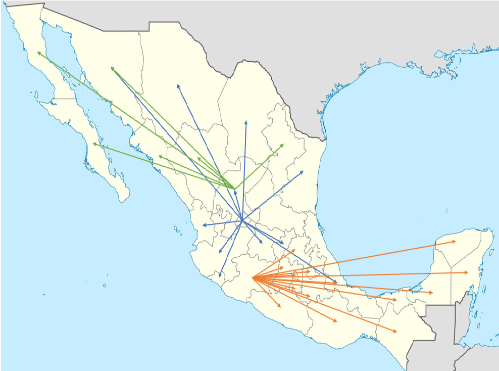
The state of Aguascalientes, mostly distributes to Jalisco 19.49%, followed by 18.26%, to Veracruz, 15.95% to Guanajuato and to lesser part with 2.12% to Nayarit, 1.38% Colima and 0.83% to Sonora. This state has a surplus of more than 5 243.79 tons that can be used to export or transform.

As for the state of Michoacán, their demands with minor participation are the states of Campeche, Tlaxcala, Quintana Roo and Veracruz with 1.56%, 2.22%, 2.52% and 2.95%, respectively. Their states with highest demand are the state of Mexico with 27.79%, Distrito Federal 16.81%, Puebla 10.70% and Chiapas 8.71%. From this offer, can spare 214.24 tons.

Zacatecas offers its production to, Nuevo León 31.16%, Baja California Norte 21.11%, Sinaloa 18.25%, Sonora 16.01%, Durango 9.23% and Baja California Sur its remaining 4.15%. Of the total, still has73.40 tons, according to model results.

As mentioned, each of the offering states have surplus, same that have production that is used to export according to the qualities and specifications required in destination markets, which is shown in the open market model.

Conclusions

Logistics modeling is given by assigning objective mathematical functions that allows to minimize costs and maximize distribution according to amount requested by the deficiency state.

Closed market model means that only equitable nationwide distribution is made, since once obtained the results, there is surplus production of guava in the states of Aguascalientes, Michoacán and Zacatecas and that with these surplus quantities have been scheduled or supplied to all deficient states; thus having maximized distribution to minimize transportation costs.

Numerical results in closed market model, has as result that the states of Aguascalientes, Michoacán and Zacatecas are bidders with a sum of more than 205 thousand tons and the other states have a combined demand about 200 thousand tons and once obtained transportation costs for each bidder to each demand on the linear programming through programming language LINDO 6.1, the costs of optimal transport is more than 78 million pesos, supplying nearly 200 thousand tons missing in other states, but an excess of 5 000 500 tons even after supplying all states, same that can be to send export or for shipment to the industry for processing into various products.

From the bidders states, Aguascalientes sends its surplus to 11 central and northern states, while Michoacán makes sends to 14 central and southern states with more than 104 thousand tons and Zacatecas sends about 30 thousand tons to 6 northern states.