Weather information

Daily information on 999 meteorological stations network INIFAP was used for a period of three years, this period was considered uninterrupted information; this network covers primarily agriculturally important regions in different agro-ecological zones of Mexico. The variables used were: maximum and minimum temperature, shortwave radiation and wind speed. The spatial distribution of the station network of the study area is presented in Figure 1.

Figure 1 Spatial distribution of 999 automatic weather stations in Mexico. 

Model FAO-Penman-Monteith

There are different models for determining ETO, each with different degree of precision and their use depends primarily on the ultimate goal of the data and weather information available. Currently, the only accepted model and standardized universally to estimate this meteorological parameter is the Penman-Monteith modified by FAO (FPM), this model was validated and endorsed by the International Commission on Irrigation and Drainage (DNIC) and the World Meteorological Organization (WMO) (^{Allen et al., 1998}) and has been used in a number of researches globally (^{Sheng-Feng et al., 2006}; ^{Gao et al, 2009}; Liu et al, 2012; ^{Chávez et al., 2013}). The FPM algorithm for obtaining the ET_O and each of the parameters required is described below:

Where: R_n is the net radiation at the surface of the reference crop (MJ m^-2 day^-1); G is the heat flow from the soil (MJ m^-2 day^-1); T the average air temperature at two meters height (°C); u2 wind speed at two meters height (ms^-1); e_s- e_a vapour pressure deficit (kPa); A slope of the vapour pressure curve (kPa °C^-1); and y the psychrometric constant (kPa °C^-1).

According to the methodology of the manuscript 56^th of FAO, there are a number of methods for calculating each of the parameters required by the previous model, these are:

Atmospheric parameters

The psychrometric constant (γ)

The psychrometric constant influences the rate of evaporation and reference crop evapotranspiration, mainly in highlands due to low atmospheric pressure. This atmospheric parameter is obtained with:

Where: γ is the psychrometric constant (kPa °C^-1); P atmospheric pressure (kPa); X constant (2.45) of the latent heat of vaporization (MJ kg^-1); C_p specific heat at constant pressure (1.013*10^-3) (MJ kg^-1 °C^-1); and 8 quotient of the molecular of steam/dry air (0622).

Also P is estimated with:

Where z is the heigth above sea level (m)

Average pressure of vapour at saturation (es )

The day value of this variable is estimated based on the temperature of the air, thereby the upper and lower temperature limits are used by the expression (^{Caí et al., 2007}):

Wher: e°(T) is the saturation pressure of steam at a temperature of specific air (kPa), T is the air temperatura (°C).

This model is applied for the maximum and minimum temperature of the day, for this reason two values for the saturation of vapour pressure are obtained and then obtaining an average value (^{Allen et al, 1998}).

Where: e _s is the average day pressure of vapour saturation (kPa); e^°(Tmax) and e^°(Tmin) are the vapour pressure at saturation at the maximum and minimum temperature, respectively (kPa).

Actual vapour pressure (ea )

The actual vapour pressure is the vapour pressure of the air when it is saturated. A saturated environment is associated with the formation of dew, hence to estimate the pressure in these conditions, dew point temperature is used. However, dew forms on the lowest (minimum) temperatures of the day, so the latter parameter (T_min) is a good estimate of the actual vapour pressure of day (^{Allen et al., 1998}; ^{Caí et al., 2007}) calculated with:

Where: e_a is the true vapour pressure (kPa); e° (T_min) is the vapour pressure at the lowest temperature (kPa); and T_min is the minimum air temperature (°C).

Solar radiation parameters

Extraterrestrial radiation (Ra )

The daily extraterrestrial radiation is calculated with the equation of ^{Duffie and Beckman (1991}):

Where: R_a is the extraterrestrial radiation (MJ m^-2 day^-1) is the solar constant (0.0820 MJ m^-2 min^-1); d_r the inverse relative distance from the earth to the sun (dimensionless), co_s the hour angle of radiation at sunset (rad); and ( the latitude (rad) and 5 the solar declination (rad).

Net radiation was calculated from the difference between the net shortwave radiation and net long-wave radiation through:

Also R_n= (1 - a)R_s where R_ns is the net shortwave radiation (MJ m^-2 day^-1); R_s already described; and a is the albedo of the reference surface whose value in this study was 0.23. On the other hand.

Where: R_nl is the net longwave radiation (MJ m^-2 day^-1); o is the Stefan-Boltzmann constant for a day (4.903 x 10^-9 MJ K^-4 m^-2 day^-1); T_maxk and T_minjk are the maximum and minimum air temperature during the day, respectively (°K); ea is the true vapour pressure (kPa); Rs as defined already; and Rso is the solar radiation on a clear day (MJ m^-2 day^-1) obtained with:

Where: z is the elevation of the station site (m); and R_a as already defined.

Monthly ET_O Behaviour

The Figure 2 shows the spatial variation ofmonthly reference evapotranspiration over Mexico, this variation is due to the combined effect of meteorological variables that affect it; mainly net radiation, relative humidity and wind (^{Xu et al, 2006}). In November the lowest values begin to lie to the northeast and northwest of the country and in States of the GulfofMexico; while high values are set in the north-central, central and some States of the Pacific coast. In December the lowest values completely cover the north and also to the States of the GulfCoast (from Tamaulipas to Quintana Roo) and only a small portion in the western States. January and December showed significant similarities with high values in the north and Gulf States, this similarity is attributed to the misuse of other meteorological parameters that directly affect the ET_O.

Figure 2 Monthly spatial variation of the ET_O in Mexico 

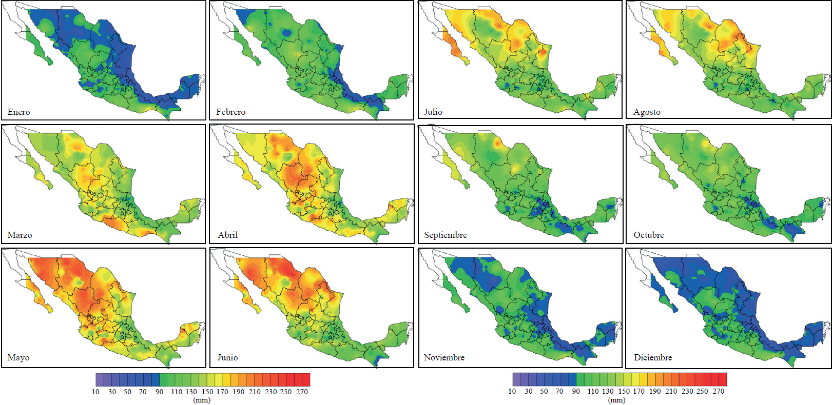
February and March show a transition behaviour between months with low values (winter) and months with high values (spring and summer), these months do not have a defined spatial pattern but significant increases in the monthly amount. The most substantial changes are observed from April, and the highest values are distributed in the north while the lower south and southeast of Mexico, this trend continues until October which coincides with results ofother researchers (^{Campos, 2006}).

The linear regression analysis between monthly ET_O and latitude indicated positive correlation from febrary to October and negative from November to January, which reflects the strong relationship between Rn and latitude and during the warmer months (^{Allen et al., 1998}). The analysis with the length showed negative correlation in the twelve months of the year; while the altitude was positively correlated from January to June and from October to December; and negative from July to September. The results of these tests are consistent with reports of other authors (^{Dalezios et al., 2002}; ^{ElNesr et al., 2010}). The correlation coefficients ofthe regressions between ET_O and geographic parameters are presented in the Table 1.

Table1. Correlation coefficients between ET_O and geographic parameters 

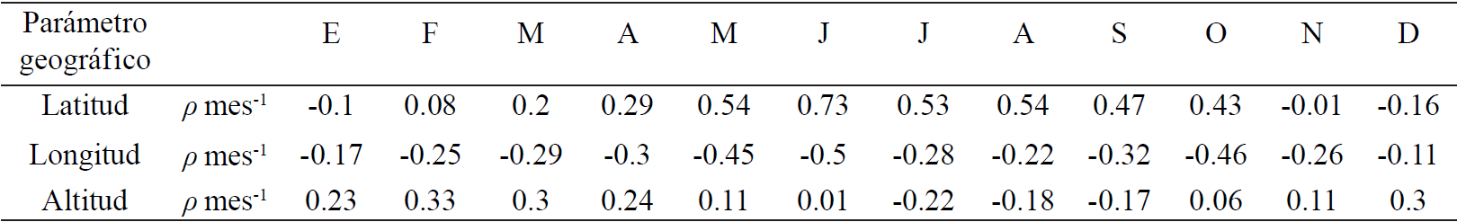
P Coeficiente de correlacion (rho)

The trend of ET_O in the year is similar in most of the study area, the absolute minimum for each station were in December and sometimes January. From December or January for some areas, ET_O begins to increase towards the spring as a result of heating the air which in turn is a result of increased R_n (Figure 3); ET_O increases toward the monthly maximum that depending on the region occurs between April and July (^{Campos, 2006}); thereafter there is a gradual decrease due to the decrease in the intensity of Rn which is received by day. However, some localities have a positive peak in August because in that month the intraestival drought, period characterized by high temperatures, sunny days and dry days mainly in climates of tropical or close to it (^{Velázquez, 1994}); after that period, ET_O resumes its descent into the winter months (^{Ruíz et al., 2011}). The trend of ET_O throughout the year is quite similar to the tendency Rn which is the main source of energy that promotes it, which is why many authors use Rn as a reference, making it into sheet of water through the factor λ (^{Allen et al., 1998}).

Figure 3 Accumulated monthly ETo and average daily Rn into two agro-ecological zones of Mexico. 

Annual behaviour of ETO

The spatial variation of the annual aggregate value of ET_O can be seen in the Figure 4. The regions with lower values are mainly oriented towards the Gulf of Mexico, distributing northwest, west, east and south of Veracruz; in this State the lowest value of the country was found (634 mm) in the experimental field station Teocelo where the currents influence of air loaded with moisture coming from the coast, another factor is the high rainfall of the area (^{Díaz et al., 2006}; ^{Granados et al., 2014}). Low values of ET_O were also presented southwest of Tabasco bordering with Chiapas and is due to high humidity reasons, noted in agroclimatology studies (^{Ruíz et al., 2012}).

Figure 4 Spatial variation of accumulated annual ET_O. 

In Chiapas these values are concentrated to the southeast and west where the relative humidity plays an important role mainly due to the high rainfall in most parts of the year in areas surrounding the dam Netzahualcóyotl and Motozintla (^{Serrano et al., 2006}). These low annual values of ET _O are presented in colours slightly purple to blue highlighting that it is relatively small compared to the total surface area of the country.

Meanwhile, the highest annual values of ET_O are located north of the republic, mainly in the States of Coahuila, Chihuahua, Durango, Baja California Sur, Sonora, eastern and northern Sinaloa; and northern Zacatecas. The maximum annual value was 1 986.15 mm in the station Empacadora de Melon (Coahuila). These high values of ET_O are associated with desert regions, mainly those located in the north-central region. These desert regions coincide with areas where the winds flow to the Pacific coast displacing atmospheric moisture of the land surface while introducing dry air from the deserts ofthe southern United States as explained by the model of atmospheric circulation of the three cells (^{Oliver, 2005}; ^{Sánchez, 2005}).

The areas of highest ET_O in the northern Mexico, coincide with the highest radiation values identified by ^{Campos (2006)} . Some areas of high ET_O are also found in isolated parts such as the State of Guerrero, northern Nuevo Leon and northeast of Tamaulipas, south of Puebla, south and southeast of Michoacán, north of Campeche and central parts of the republic (northeast Jalisco, much of the State of Guanajuato, east and northeast of San Luis Potosí, and Tlaxcala center). In the Figure 4, we can see that values of ET_O in the range of1 536 to 1 986 occupy most of the area under study which is consistent with reports of ^{Medina et al. (2006}) who points for these regions the highest rates of aridity and drought.

Regarding low annual values of ET_O and high values in rainfalls, there are positive water balances, where soil moisture leads to at least one crop cycle per year, in there the crop water requirements are met by rainfall and storage capacity of water in the soil (^{Eldin, 1983}). While in the regions where ET_O is higher than precipitation, as in arid areas, irrigation of crops is necessary to obtain commercial crops; there, the ET_O provides great support for the design, planning and management of irrigation (^{Chávez et al., 2013}). The maps in Figures 3 and 4 provide useful information for planning and water management at the basin level, since monthly or annual values of ET_O is an important parameter in the hydrological cycle because they represent the upper and lower limit in the evapotranspiration demand of the atmosphere at different sites (^{Xu et al., 2006}).