


 nova página do texto(beta)
 Inglês (pdf)
 Artigo em XML
 Referências do artigo
 Enviar este artigo por email
 Citado por SciELO
  Similares em
SciELO
Similares em
SciELO 
 Permalink
Introduction
The finite element method is one of the most popular general purpose techniques for computing accurate solutions to partial differential equations (pdes). Since pdes form the basis for many mathematical models in the physical sciences and other fields, it is not hard to realize the importance of the finite element method. The finite element method reduces a boundary value problem for a partial differential equation or system of pdes to a system of linear equations, written in a matrix form KU=f that can be solved numerically. In many cases the stiffness (K) matrix is symmetric and sparse, with the sparse structure highly influenced by the node (nodal finite element method [21], edge (edge elements [10]), and element (discontinuous finite element method [4, 3]) numberings provided by the grid generator.
Here, sparse matrix techniques are preferable since the storage required increases as 0 (N) where N denotes the degrees of freedom of the problem. Storage can be reduced by storing only the nonzero elements with a compress sparse row format. Sparse matrix-vector multiplication is an important kernel in many iterative solvers; with parallel implementations
We can obtain a solution in a reasonable amount of time but they suffer from low cache utilization due to unstructured data access patterns. [7, 2] proposed to reorder sparse matrices using a bandwidth reduction technique in order to reduce the number of cache misses to improve the memory-system performance of the sparse matrix-vector multiplication. Sometimes it is not easy to assemble the stiffness matrix and reorder its elements since the matrix is assembled at running time, or if it is too large it must be split among different processors. Here we discuss how to use RCM to reorder nodes, edges and elements of the mesh in order to reduce the bandwidth of the assembled matrices. The work is organized as follows: section 2 introduces the edge- and element-defined finite element formulations employed, in section 3 the different meshes used in our numerical computations and the influence of the edge and element ordering in the sparse structure of the finite element matrices are presented, then section 4 introduces the RCM renumbering of edge and elements graphs, with some numerical experiments also included, and finally section 5 establishes the conclusions of this work.
Finite Element formulations
Edge-element formulation
For the edge-element formulation let us consider the problem of calculating resonant frequencies of cavities ([8, 1]). The nodal formulation is:
Where
The finite element formulation is given by
The electric field in a single triangular/tetrahedral element is represented as
Here
Discontinuous formulation
For discontinuous formulation ([4], [3]) we consider the conservation laws
At each time t∈[0, T] the approximate solution is sought in the finite element space of discontinuous functions
Where τh is the triangular discretization of Ω, P(k) is the local space of polynomials of degree ≤ k. The weak formulation of (4) is
Where ψ is a smooth function, n is the outward unit normal to face e of element T. In the above expression we replaced u by its approximation uk, the first two terms correspond to volume integrals, and the last term requires the evaluation of numerical fluxes.
Sparse Structure and Bandwidth of Finite Element Matrices
Meshes
The most popular element shapes employed for two and three dimensional applications are triangles and tetrahedra respectively; this is due to the fact that they are the simplest tessellation shapes for modeling arbitrary two and three dimensional geometries and they are also well suited for automatic mesh generation. To investigate the influence of the edge and element numbering in the structure of the stiffness matrix, we employ the grid generators Triangle [18] and Tetgen [19], which are two and three dimensional mesh generators that use Ruppert’s Delaunay refinement.
These grid generators, in addition to providing nodes and elements, compute edges and neighbors of the elements (which is very convenient for element-defined and edge-defined finite element formulations).
We consider two simple geometries; for the two-dimensional case a circle with three interior circles removed, and for the three-dimensional case, a cylinder with three interior cylinders removed. An unstructured triangular mesh is generated by Triangle, whereas an unstructured tetrahedral mesh is obtained with Tetgen. Figures 1-2 show with a few elements the meshes considered. Also Figure 3 shows a two-dimensional view of the three-dimensional domain.
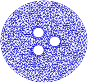
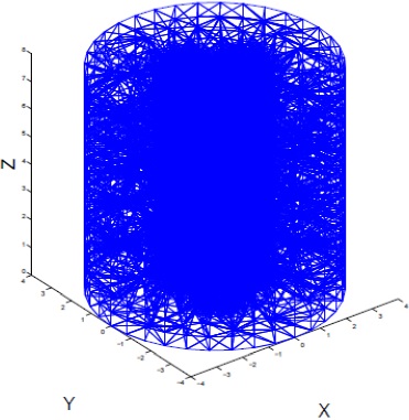

Table (1) shows the information for the meshes. Here n-nodes, n-elements and n-edges denote number of nodes, elements and edges respectively.
Sparse Structure of edge-defined and element-defined formulations
In this section we discuss how the numbering of edges and elements affect the sparse structure of the stiffness matrix.
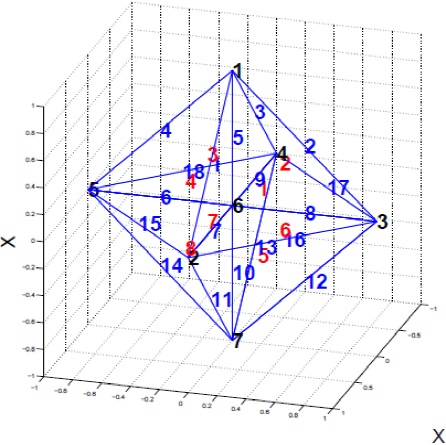
The structure of the three-dimensional case is discussed in detail and some notes are stated for the two-dimensional case. Let us introduce the following 3d sample mesh.

This mesh file contains information of nodes, elements and edges. It can be obtained from the node, element, edges, and neighbors files provided by the grid generator Tetgen (two-dimensional versions of these files can be obtained by using Triangle). Its first line contains n-nodes, n-element and n-edges (number of nodes, elements and edges respectively), the following n-nodes lines contain the nodes coordinates (two or three), and the next n-elements lines contain the element node connectivity (nodes that define each element).
For triangles there are three nodes, a boundary marker and its three neighbors. For tetrahedral: four nodes, a boundary marker and its four neighbors. Finally n edges lines that contain the nodes that define each edge. Figure (4) shows the 3d simple mesh with its nodal, edge and element numberings.
In order to assemble the stiffness matrices in nodal, edge and element formulations we need the corresponding element-node, element-edge and element-neighbors connectivity Tables. The element-node and element neighbor’s Tables are obtained directly from the mesh files, but the element-edge needs to be computed from the element node connectivity and the list of edges. In [14] two methods to compute an element-edge Table were discussed.
Let us start our discussion of the assembly process considering first the nodal case with linear elements. In the literature there are several works reporting how the RCM reordering has been applied to the nodal case, and we mention it here for completeness of our discussion; from the element to node connectivity Table provided by the grid generator we can get the structure of the finite element matrix K. A loop over the n elements rows of this Table says that for the row i the matrix K has nonzero elements on K (table(i,1), table(i,2)), K (table(i,1),table(i,3)), K (table(i,1),table(i,4)), K (table(i,2),table(i,3)), K (table(i,2),table(i,4)) and K (table(i,3),table(i,4)), where of course we have to take into account the elements of the diagonal (each node is related to itself) and the symmetries of the matrix.
Table 2 Element to node connectivity Table of our 3d sample mesh.
| 1 6 2 3 |
| 1 6 3 4 |
| 1 6 4 5 |
| 1 6 5 2 |
| 3 6 2 7 |
| 4 3 7 6 |
| 5 4 7 6 |
| 2 6 5 7 |
Now for the edge-element formulation with linear elements, the finite element matrix can be built in a similar way as it was built in the nodal case. Here an element-to-edge Table is required. Table 3 shows the element-to-edge connectivity Table for the sample mesh. The last six columns contain the numbering of each element-edge. A loop over the n-elements rows of this element-edges Table says that for the row i the matrix K has nonzero elements on K (table(i,1),table(i,2)), K (table(i,1),table(i,3)), K (table(i,1),table(i,4)), K (table(i,1),table(i,5)), K (table(i,2),table(i,3)), K (table(i,2),table(i,4)), K (table(i,2),table(i,6)), K (table(i,3),table(i,5)), K (table(i,3),table(i,6)), K (table(i,4),table(i,5)), K (table(i,4),table(i,6)), K (table(i,5),table(i,6)), where we also consider the elements of the diagonal (each edge is related to itself) and the symmetries of the matrix.
Table 3 Element to edge connectivity Table of our sample mesh.
| 1 6 1 2 1 3 2 6 2 3 3 6 | 5 | 1 | 2 | 7 | 16 | 8 |
| 1 6 1 3 1 4 3 6 3 4 4 6 | 5 | 2 | 3 | 8 | 17 | 9 |
| 1 6 1 4 1 5 4 6 4 5 5 6 | 5 | 3 | 4 | 9 | 18 | 6 |
| 1 6 1 5 1 2 5 6 2 5 2 6 | 5 | 4 | 1 | 6 | 15 | 7 |
| 3 6 2 3 3 7 2 6 2 7 6 7 | 8 | 16 | 12 | 7 | 11 | 10 |
| 3 4 4 7 4 6 3 7 6 7 4 6 | 17 | 13 | 9 | 12 | 10 | 8 |
| 4 5 5 7 5 6 4 7 6 7 4 6 | 18 | 14 | 6 | 13 | 10 | 9 |
| 2 6 2 5 2 7 5 6 5 7 6 7 | 7 | 15 | 11 | 6 | 14 | 10 |
At [14] the local number of edges is specified and also more implementation details are included.
Finally in an element wise finite element formulation (finite volume or high order discontinuous Galerkin); we need the neighbors of each element. Table 4 shows the element to node connectivity Table with their four neighbors (three for triangles) for the 3d sample mesh. Here a zero means that the element does not have a neighbor (its edge/face is on the boundary). From the element to neighbors connectivity Table we can get the structure of the finite element matrix K in the discontinuous case; a loop over the rows of the Table says that for the row i the matrix K have nonzero elements on K (i,table(i,1)), K (i,table(i,2)), K (i,table(i,3)) and K (i,table(i,4)) where of course we consider only the nonzero elements of the neighbors connectivity Table and again we take into account the elements of the diagonal and the symmetries of the matrix. Note that the numbering of edges and elements is given by the order as they appear at the files provided by the grid generators.
Reordering and Numerical Experiments
Nodal Renumbering
Traditionally, bandwidth reduction is obtained by a reordering of nodes of the finite element mesh. Some of the most common used algorithms include: Reverse Cuthill McKee [5], and Gibbs-Poole [15]. TRIANGULATION RCM and TET MESH RCM are programs which compute the reverse Cuthill-McKee reordering for nodes in triangular/tetrahedral meshes; they are freely available in C++, FORTRAN90 and MATLAB versions [12]. The nodal renumbering scheme is directly applied to the node graph. It is desirable that grid generators incorporate node renumbering algorithms.
Edge renumbering
In ([13, 14]) two edge-numbering schemes provided by Jin [8] were tested for two- and three-dimensional implementations respectively. Numerical experiments there showed that if the node labels are close enough, a good edge-numbering scheme (low bandwidth) can be defined by using an indicator to each edge (the indicator was i1 × i2 with i1 and i2 denoting the end nodes of the edge) with the array of indicators rearranged by a sorting algorithm very similar to the edge-reordering scheme used in [6]. In this work we use a different approach. Our starting point is any edge numbering, for example the one provided by Tetgen or Triangle.
To fix the ideas, let us refer to our 3d sample mesh from Figure 4. The last six (three for triangles) columns of element-to-edge connectivity Table (3) define the connectivity of what we call the Edge-Graph. A graphical representation of this mesh can be generated by joining the middle points of edges of the original Node-Mesh, Figure 5 shows this graph. This is our main contribution; because once we have defined the connectivity of the Edge-Graph we proceed to apply a renumbering algorithm as RCM.

Elements Renumbering
For the discontinuous formulation, in addition to the description of the elements by the connectivity of their nodes, a list of the neighbors of each element is required. Both grid generators Triangle and Tetgen provide the neighbors for triangles and tetrahedra respectively. In our 3d sample mesh, the last four (three for triangles) columns of Table (4) define the connectivity of what we call the Element-Graph. This is our main contribution because once we have defined the Element-Graph we can apply the renumbering algorithm to its connectivity Table. Notice that we can generate its graphical representation by joining the barycenters of the elements of the original node graph. Figure 5 shows this graph.
Numerical Experiments
We use meshes generated by the grid generators Triangle and Tetgen to assemble the matrices for the edge and discontinuous formulations given in section 2.
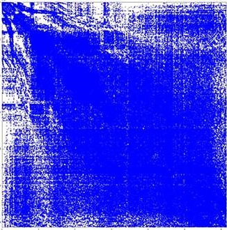
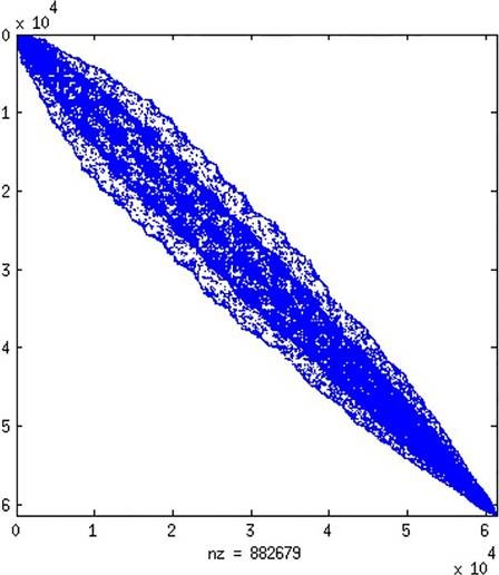
Let us make some comments about the edge-element formulation. Figure 6 shows a sparse matrix structure obtained by using the original edge-numbering provided by the grid generator [14], whereas the matrix structure showed at Figure 7 was assembled using a node-reordered mesh (RCM) followed by the S1 edge-numbering scheme, and finally the matrix structure showed in Figure 8 was assembled using the RCM applied to the Edge-Graph. As mentioned in [14], scheme S1 is a good edge-numbering provided the nodes are close enough numbered, but the best result is obtained by directly applying the RCM reordering to the Edge-graph. In fact, after using a node-reordered mesh with the edge-numbering S1 the original bandwidth was reduced in a 332%, but when a RCM-renumbering is directly applied to the edge graph the bandwidth is reduced in a 610%.

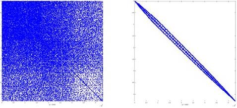
As it has been widely reported, RCM applied to nodes of a mesh reduces the bandwidth of assembled matrices in nodal finite elements formulation. In order to obtain a bandwidth reduction in finite volume or discontinuous Galerkin formulations, we defined the Element Graph and applied the RCM reordering of elements. Figures 9 shows the sparse matrix structure for the element-defined formulations for both the original tetrahedral mesh and the graph element RCM reordered.
We observed similar results in two and three dimensions for nodes and elements.
Figure 9 shows the sparse structure of the matrix of the element wise finite element formulation for the original numbering of the elements and the RCM reordering of the elements graph.
In time domain formulation with edge-elements to simulate transient electromagnetic fields in 3d diffusive earth media [20] and high-order Navier-Stokes simulations using a Discontinuous Galerkin Method [17] both of them reduce to a sparse-matrix-times-vector product operation employed by the time solvers. Thus, a simple OpenMp code was implemented to multiply the assembled matrix sparse storage times a vector, and the execution time is reported.
void SPARSE::Matrixvector(real vect[],real vectprod[])
{
long long int k;
unsigned int i;
int chunnk=1000;
{
#pragma omp for private(k,i) schedule(static,chunk)
for ( i = 0; i ¡ dim; i++)
{
vectprod[i]=0.0;
for ( k = IA[i]; k ¡ IA[i+1]; k++)
vectprod[i] += AA[k-1]*vect[JA[k-1]-1];
}
}}
Figure 10 shows the execution time of the sparse-matrix-times-vector product as a function of the number of iterations. Here original refers to edge-numbering provided by the grid generator whereas reordered refers to the reordered edge graph. For iterations between 200 and 600 the execution time is reduced by an average of 27.5%. The OpenMp code sparse-matrix-times-vector products were performed in an Intel Core CPU 2.90 GHz 8 processors workstation. Figure 11 reports execution times for both the originally numbered and the reordered element-graphs corresponding to the element-wise formulation. It is desirable that grid generators include the RCM renumbering for nodes, edges and elements in order to avoid the post processing of the mesh or the reordering of the assembled matrix in the different finite element formulation. The bandwidth reduction obtained by edge or element reordering reduces the cache misses, improving the execution time of the sparse-matrix-vector product which is the main kernel of iterative solvers as BCG, QMR, etc. [11]

Figure 10 Matrix times vector execution time as a function of the number of iterations, edge elements formulation.

Conclusions
Bandwidth reduction of matrices produced by nodal edge and element-defined finite element formulations were obtained.
To apply a renumbering scheme like RCM (originally designed for nodal) we have defined the N and Element-Graph. The optimal mesh obtained (node-reordered, edge-reordered, and element-reordered) can be very valuable. Some methods, for example those that combine nodal and edge-defined finite element formulations [9] or those that combine nodal finite element and finite volume methods [16] could directly benefit from these reorderings. We suggest that grid generators should incorporate nodal, edge and element renumbering of the produced meshes in order to reduce bandwidth of assembled finite element matrices, avoiding the preprocessing of the mesh or the post processing of the assembled finite element matrix (sometimes quite difficult because the matrix is assembled at execution time or distributed over different processors). Moreover, the bandwidth minimization renumbering scheme that has been discussed reduces the cache misses improving the execution time in the sparse-matrix-times-vector product implemented on OpenMp. Matrix-vector multiplication is one of the main kernels in the iterative solvers. In this work we have discussed first order nodal and (CT/LN) edge finite elements, and a future work is due to investigate high order nodal and edge elements beside extended stencil finite volume formulations (extended neighborhoods for high order finite volume formulations).

