


 text new page (beta)
 English (pdf)
 Article in xml format
 Article references
 Send this article by e-mail
 Cited by SciELO
  Similars in
SciELO
Similars in
SciELO 
 Permalink
Introduction
About 80% of Mexican energy consumption comes from fossil fuels, including that of the whole transportation sector (SENER, 2018). This makes the country the 13th largest Greenhouse Gas (GHG) emitter in the world, contributing with about 1.5% of the global GHG emissions (The World Bank, 2018). The country’s environmental goals, in accordance with the Intended Nationally Determined Contribution, require that 35% domestic energy should come from renewable sources by 2024 and a 22% GHG reduction by 2030 with respect to a business-as-usual scenario. Meeting these goals is likely to require a domestic biofuel industry. The 2013 energy reform, however, was mostly designed to increase fossil fuels production in the transportation sector (Fernandez Madrigal, 2015), and the new proposed counter-reform goes in the same direction in these respects (SENER, 2020).
There have been several attempts to introduce biofuels into the market. The most recent plan was to require gasoline be blended with 5.8% bioethanol (hereafter referred as ethanol) in all the country but the three main metropolitan areas1, but so far, no success, and it is not in the top priorities of the current federal administration. Anecdotal evidence suggests potential producers are unwilling to bear the fixed costs of setting up production systems because they doubt policies will endure. There has been a surplus of sugarcane in several recent years, but no industrial-scale fermentation or distillation facilities to turn it into ethanol. Thus, it is required that whatever policies the country implements to promote biofuels be seen as sustainable. This article is aimed directly at that goal, developing a framework to project and assess policy impacts on the biofuel market in the following years.
According to Rendon-Sagardi et al. (2014) there is an interest by the Mexican government for the development of a domestic biofuel industry, in particular to promote the growth of second and third-generation biofuels. However, efforts have not been enough, since currently biofuels replace only 0.8% of domestic demand for fuel, and not necessarily in the transport sector. This low rate of participation can be attributed to the low costs of fossil fuels. Ethanol can become almost twice as expensive than the average cost of gasoline imported by Mexico, which makes difficult to develop an economic and sustainable domestic biofuel industry (Maldonado-Sanchez, 2009). So this research provides additional analysis to assess the potential of the domestic biofuel industry and how it can evolve in the international markets, given that Mexico shares a long land border with the world largest biofuel market.
Mexico is the fourth largest economy in the West hemisphere, after the U.S., Canada, and Brazil (The World Bank, 2018), but México is the smallest biofuel producer in the region, while the U.S. and Brazil are the first producers worldwide (EIA, 2019). The U.S. developed its biofuel industry, in particular the ethanol one, since 2005 thanks to setting ambitious goals of fuel mixes (136 billion liters to be mixed by 2022), along with tariffs to imported biofuels and tax credits to biofuel producers (EPA, 2010). Brazil build this industry in an longer period, since 1975 when the Brazilian government embarked on an ambitious program known as Programa Nacional do A´lcool to produce large quantities of ethanol from biomass (e.g. sugarcane, cassava and sorghum) as a substitute for gasoline by providing economic incentives to ethanol producers and consumers. For a variety of reasons, including low international prices for sugar and idle capacity for distillation, sugarcane became the sole source of ethanol. After several years of a significant production, it came down throughout the 1990s, in part due to the elimination of subsidies and price supports, the deregulation of the ethanol industry, low international crude oil prices, high sugar prices in world markets, and oil discoveries off the Brazilian coast (Rosillo-Calle and Cortez, 1998; Salvo and Huse, 2011). It was only in March 2003, when the Brazilian automotive industry introduces to the market of the flex-fuel vehicles, which are capable of running on any blend of gasoline and hydrous ethanol. Along with this new technology, both federal and states governments have provided lower tax rates to ethanol relative to those on gasoline, which have boosted domestic ethanol consumption in the last decades. These two are good near examples of policy perseverance, which has not been the case of México. Hence, the normative analysis in this paper may help policy makers to assess policies used in other countries and how they would result in México.
Technically, an endogenous-price mathematical programming partial equilibrium model is developed emphasizing the Mexican agricultural and fuel sectors, which are embedded in a multi-country, multi-region, multi-product, spatial framework. Biofuel could be produced both from dedicated crops and from agroindustrial residues. In the model, ethanol production is only allowed from sugarcane and agave industries. The model assumes all markets are competitive so that the economy maximizes the sum of producer and consumer surplus subject to resource limitations, material balance, technical constraints, foreign offer surfaces and policy restrictions. Although competitive markets can be a strong assumption since the Mexican fuel market is dominated by the state-owned oil company (PEMEX), the 2013 energy reform allowed the entry of private gas stations to the market so they compete with PEMEX gas stations. As 2021, approximately 23% of the market has been taken up by private gas stations. As such, the model allows a competitive market for the fuel final user as well as ethanol.
This article contributes to the understanding of the interactions between food, feed, and fuel sectors under policy and technological changes in Mexico. In particular, the model considers three policy alternatives as well as a base case in which, as now, no policy is intended to promote ethanol. The first alternative consists of subsidies to ethanol producers, the second of blending mandates and the third of both combined. For the scope of this article, the optimization considers only two specific values for the policy parameters. Ethanol international trade is allowed in all three cases.
Projecting market conditions to 2025, which is an achievable goal for the biofuel industry, results show that domestic production would be low under all scenarios, and rather this type of policies will incentive ethanol trade with the U.S. In addition, the model results show some losses for fuel and agricultural consumers, that are not offset by both ethanol producer and GHG emissions reduction gains. Most of that benefit will be enjoyed abroad because a subsidy by itself will be transferred abroad in form of ethanol.
The next section provides a brief methodological literature review as well as a revision of the works done for Mexico. Following that the model, the data, and assumptions underlying the analysis are described. A description of the results and policy implications concludes the article.
Literature Review
A rapidly growing literature on the economics of biofuels discusses the scope of land use changes and policy distortions. Rajagopal and Zilberman (2007) provide a review of literature on analysis and modeling aspects of biofuels policy. A more recent review of the literature on modeling aspects can be found in Khanna et al. (2011). The model developed here follows the modeling strategy of a larger and known sectoral partial equilibrium model: FASOM (Forest and Agricultural Sector Optimization Model), which is utilized to evaluate agricultural and environmental impacts of the U.S. Renewable Fuel Standard (RFS) against a scenario with a low production of biofuels (Beach and McCarl, 2010). The FASOM is a programming model of endogenous, multisectoral, dynamic, non-linear developed for the U.S. agricultural sector prices. The model uses the approach of maximizing social surplus to determine the simultaneous equilibrium in the markets for agricultural products, disaggregating both the agricultural sector in several major producing regions within the U.S. (McCarl and Spreen, 1980; Norton and Schiefer, 1980; Takayama and Judge, 1971).
Following a similar strategy, Chen et al. (2011) develop BEPAM (Biofuel and Environmental Policy Analysis Model) to evaluate the change in land use and prices of food and fuel due to U.S. biofuel policies, compared to a stage without any intervention. BEPAM is an endogenous, multisectoral, dynamic, programming model that also uses the approach of welfare maximization. The authors argue that the subsidy to produce second-generation ethanol is necessary to fulfill the mandate of cellulosic biofuels.
With regards to the partial equilibrium models that consider emerging economies, most of them has focused on the Brazil market (e.g. Elobeid et al., 2011; Nassar et al., 2009; Fabiosa et al., 2010). For example, the authors assess all the spectrum of policies in Brazil to modify the ethanol market in Brazil, that is different mandate rates (15% to 30%) as well as different rates of reduction to fuel taxes (from 0% to 100%), aiming to indicate and quantify the implications of alternative choices under different market conditions and the socioeconomic objective(s) of the public policy makers.
For the Mexican case, it has not been developed a model as those described above for the U.S. and Brazil. However, some stylized models, descriptive studies and cost-benefit analysis can be found in the literature (e.g. Sanchez et al., 2013; Sanchez and Gomez, 2014; Sanchez et al., 2016). According to the simulation made by Rendon-Sagardi et al. (2014) is expected fuel demand to increase by almost 60% from 2014 to 2030. The authors point out that this will represent a problem for the expected decline in domestic production oil: today, national proven reserves cannot guarantee self-sufficiency. Under this scenario, Rendon-Sagardi et al. (2014) found in biofuels a possible exit to this problem. In this sense, the choice of biofuels is potentially important in Mexico since it is the third largest agricultural producer in Latin America, which is reflected in the approximately 75 million tons of dry matter generated by 20 major crops in the country. Of these, corn stover, sorghum and wheat straw, as well as leaves of sugarcane rep resent more than 80% of that dry matter while the rest is mainly bagasse from sugarcane, corn cob and coffee pulp (Valdez-Vazquez et al., 2010). In this context, in recent years they have tried to promote policies that encourage the use and development of renewable energies such as the development of technologies to obtain second-generation biofuels (either through combustion or fermentation). Valdez-Vazquez et al. (2010) explore the location and amounts of crop residues that could be used in the production of second-generation biofuels and find that there are municipalities that could reach production of 0.3 million liters of ethanol per year (by anaerobic fermentation).
Sugarcane is the crop that has emerged as the most promising crop in the medium and long term, regarding the production of ethanol, even above the corn (SENER et al., 2006). Sugarcane ethanol, however, could be profitable only under certain economic conditions (SENER et al., 2006), but not a complete study of the sugarcane market has been done to evaluate its viability. A second and relevant source of biomass is the agave, which is primarily used for tequila and mezcal production, and turns out to be less expensive than sugarcane because of its low water demand, less need for fertilizers and their ability to grow in semi-desert areas with lower quality soil. The agave and spirits industry residues have been the subject of significant research and are considered to have high potential as biofuel feedstock (e.g. Munoz et al., 2008; Cáceres-Farfán et al., 2008; Maldonado-Sánchez, 2009; Davis et al., 2011). A study of cost-benefit by Maldonado-Sánchez (2009) find the sugar content of agave to be greater than that of sugarcane or yellow corn from the U.S. Also, the authors point out that production of biofuels from agave does not compete directly with the distillation of drinks as for the generation of biofuels is to use the waste of agave resulting from the production of tequila and mezcal. Additionally, the authors argue that, with higher conversion efficiency or using sugar that is present in other parts of the plant (reaching up to 212 metric tons per hectare), can reduce the cost to $0.6 per liter, which would make it competitive with ethanol made from corn or sugarcane.
At this point, the U.S. RFS can play an important role to develop ethanol industry in Mexico. The RFS aims to increase the amount of biofuels blended with conventional fuels to 136 billion liters by 2022. An important component of this target is the ‘advanced’ biofuel mandate , which is set as 79 billion liters for 2022. According to the RFS provisions, at least 60 billion liters of this amount must be derived from cellulosic biomass while the rest can be met by biodiesel and sugarcane ethanol. Due to the slow progress in advanced biofuel production, part of it could be met by sugarcane and agave ethanol imported from Mexico. If an economically competitive cellulosic biofuel technology is established by 2022 in Mexico and the RFS is maintained as originally designed, Mexico could export part of its production to the U.S. Therefore, the RFS advanced biofuel mandate may have important implications for the Mexican ethanol industry.
The relevance of this advanced mandate is explained in Figure 1, that shows intuitively some expected results under three scenarios: an ethanol mandate, a subsidy to ethanol producers, and both policies combined. Figure 1(b) shows that imposing a blending mandate shifts gasoline demand to the left, but ethanol would be imported from the U.S., so no further changes would occur in the Mexican sectors. When a subsidy is in place, it works the other way around, supply of ethanol shifts to the right, but producers prefer to export it to the U.S. that needs to satisfy the advanced mandate with the Mexican ethanol as shown in Figure 1(c). In addition, supply of sugar and spirits shifts to the left. Finally, when both policies are combined, gasoline demand shifts to the left, and ethanol can move in different directions, for instance as shown in Figure 1(d), Mexico could export the domestic ethanol production to the U.S. for the advanced mandate, and import corn ethanol from the U.S.
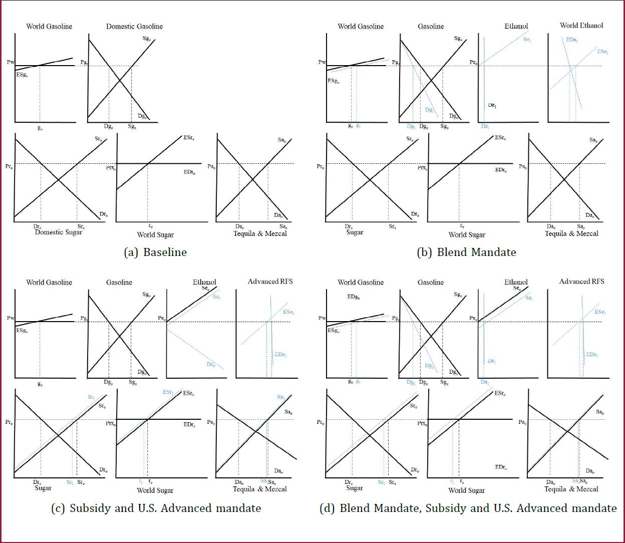
Notes: Blue lines denote the changes under each policy scenario. P denotes price, ES excess supply, ED excess demand, S supply, D demand; g denotes gasoline, e ethanol, r sugar, a spirits, w world. Sub-index o denotes the baseline set up and 1 the change under each scenario.
Figure 1 Effect of alternatives ethanol policies on the Fuel, Sugar and Spirits Sectors
This article contributes to the related literature by developing a simultaneous framework that incorporates the interactions between food, feed, and fuel sectors for analyzing the impacts of policy and technological changes on the biofuel economy and subsequent land use changes in Mexico. This article differs from the previous studies which addressed similar issues in several ways. First, to the best of our knowledge it is the first programming model developed for these sectors in Mexico. In this the model, the simulation aims to explore the potential of sugarcane and agave as feedstocks for production of first and second-generation ethanol, respectively, and for the later feedstock biomass would come from agave plant leaves and trash and agave not harvested for spirits production. The expected result is that Mexico will need high subsidies and mandate blending rates to promote ethanol and consolidate a domestic ethanol industry. The advantages of sugarcane and agave are that impacts in term of land use due to ethanol production will be small. Secondly, this article comprises an explicit fuel transportation component for Mexico that includes fuel transportation among Mexican states and fuel trade with the U.S. and the row. Finally, the model in this article includes a fuel market mechanism that will allow to understand domestic policies and pricing system more accurately, which has not been addressed in the biofuel modeling literature.
The Model
The model employs the social surplus maximization approach first introduced by Samuelson (1952) and later fully developed by Takayama and Judge (1971, 1964). McCarl and Spreen (1980) and Martin (1981)) provide a rigorous presentation of the methodology and review numerous studies that used this approach. This optimization model simulates the formation of simultaneous equilibrium in multiple markets by maximizing the social-surplus derived from production and consumption of a set of products subject to material balance equations, resource availability, and other constraints related to technical limitations. The social-surplus (quasi-welfare) function includes the agricultural and fuel markets in Mexico as well as the excesses of supply and demand from the U.S. and the row. The consumers’ surpluses are derived from consumption of agricultural commodities in all these countries, fuel consumption in U.S. and the row and Vehicle Kilometers Traveled (VKT) in Mexico. VKT demand is produced from gasoline, diesel, jetfuel, or ethanol, which in the later case can be produced from agave residues and sugarcane. For readability, this section provides an overview of the model. A detailed mathematical description is presented in the Appendix A.
As in similar models presented in the literature, the supply and demand functions are all assumed to be linear and separable. The supply response in Mexico agricultural sectors is modeled explicitly by using Leontief (fixed input-output) production functions. These assumptions imply an additive quadratic utility function that represents the sum of producers’ and consumers’ surplus in the three global regions.
The agricultural supply side of the model is regionally disaggregated at agricultural district level in the Mexico component. The comparative advantage between crop and pasture activities in each region is modeled explicitly based on the domestic and world prices, costs of production, processing costs, costs of transportation, and regional yields. The total cost of producing agricultural commodities in the 193 districts is expressed as a linear function of the areas planted assuming fixed production costs for individual crops. In the Leontief production functions used for crop production land is considered as the only primary input and crop yields are assumed as the output. The land allocated to all crops and pastures is constrained by the total agricultural land availability in each district at the base year values, while the availability of all other inputs is assumed to be unlimited at constant prices observed in the base year.
Adifficulty that is often encountered when working with programming models inagricultural sector analysis is that optimum solutions generated by the model may involve unrealistic and extreme specialization in crop production. This difficulty is addressed here by considering the ‘crop mix’ approach (McCarl, 1982; Onal and McCarl, 1991) where the land allocation and livestock heads in each region are restricted to a convex combination of the historically observed patterns in that region. To allow some flexibility beyond the historical mixes the model also incorporates ‘synthetic crop mixes’ which are generated by use of systematic hypothetical variations in crop prices and supply response elasticities (Chen et al., 2012).
The optimal output levels based on the land allocations at district level are aggregated to determine the national supply of agricultural commodities that can be consumed either in the domestic market as food, feed, or exported, all of which are driven by downward-sloping linear demand functions. For the U.S. and the row, the model assumes linear excess supply and demand curves based on the quantities traded among the three regions and the international prices. Agave biomass and sugarcane are the biofuel feedstocks considered in the model. In Mexico, the use of agave residues and the use of sugarcane as ethanol feedstock is related to the endogenously determined domestic and export demand for ethanol as well as the domestic and export demands for tequila, mezcal and sugar, respectively. Besides primary commodity demands, the model includes processed commodities from agave, soybean, and sugarcane in Mexico as well as their processing costs.
In the fuel sector, when projecting market condition to 2025 ethanol and gasoline are assumed to be substitutes within the specified blending regulations to generate blended fuel and the subsidy to ethanol producers is included in the objective function. The model assumes upward sloping supply functions for oil, gas, and petroleum products (i.e., gasoline, diesel, fuel jet, fuel oil, etc.) in the U.S. and row components, since the model works only with the demand and supply excesses. Upward sloping supply functions for oil and gas are assumed in the Mexican component, while the supply of petroleum products is driven by processing costs and the VKT market in the case of gasoline, ethanol, diesel, and jet fuel. For gasoline and ethanol, in addition to the processing cost, delivery and distribution costs from refineries, ports and storage and distribution facilities to states are also considered; and a downward sloping demand curve in the case of gas and the rest of petroleum products. Because of the long transportation distances between the potential ethanol production regions, ports and gasoline refineries and the consumption locations, a fuel transportation module is included in the Mexican component. Specifically, each of the 32 states is assigned a fuel demand function2 and the gasoline or ethanol needed in each state are first delivered from the ethanol producing districts, gasoline refineries, or importing ports to the storage points, where both fuels are mixed, and then delivered to each state at least cost. Ethanol international trade is also considered based on the total supply and demand from the U.S. and row. The model determines the optimal supply chain network simultaneously with the food and fuel market equilibrium.
Data and Assumptions
The data inputs include the base year domestic and global commodity prices and quantities de manded, historical crop mixes (areas planted to individual crops), crop yields, costs of production and processing, and cost of transportation. Crop mixes are restricted to the 2000-2013 data. Mexico is disaggregated into 193 districts. The crop sector includes: Agave tequilana Weber variety Blue (hereafter referred to as A. tequilana), Agave species for mezcal production (hereafter referred as A.mezcalero), alfalfa, barley, beans, yellow corn, white corn, corn silage, fodder grass, green chili pepper, oats, oat silage, orange, sorghum, soybeans, sugarcane, and wheat. In addition to crops, the model includes the pasture area, where cattle are raised and six processed goods: tequila and mezcal from Agaves; soybean oil and soybean meal from soybean; sugar from sugarcane; and ethanol from sugarcane and agaves’ residues.
Historical land use, crop yields and pasture areas are obtained from Servicio de Información Agroalimentaria y Pesquera (SIAP). Costs of production of the crops include variable operating costs (seed and treatment, fertilizer, hauling and trucking, drying and storage costs, interest on operating cost, limestone, chemical costs, fuel, and oil, and hired labor costs), fixed operating costs (tractor and machinery, crop insurance, marketing and miscellaneous, stock quota lease, irrigation), and capital and overhead costs. For each state, the variable operating costs and interest on investment are assumed to be yield dependent while the remaining costs are fixed. Costs of production are gathered at state level from Sistema Producto (SisProd).
When specifying the agricultural commodity demands, the model uses 2008 as the base year, the prices and quantities as reported in SIAP (2015), CRT (2015), CRM (2015), USDA-FAS (2015) for Mexico, USDA-NASS (2016), USDA-FAS (2015), Comtrade (2015) for U.S. and ROW. The price elasticities for Mexico, U.S. and ROW used in the demand functions are obtained from various sources, including USDA-ERS (2015), FAPRI (2015), Meyers et al. (1991), Rowhani et al. (2010), Euromonitor Internacional (2014), Chen et al. (2011), IndexMundi (2014), Hoffman and Livezey (1987), Summer (2003), Russo et al. (2008), Haniotis et al. (1988) Ali (2006), Brown (2010), and Vittetoe (2009). For fuels, elasticities where also gathered from different sources (e.g. Galindo, 2005; Crotte et al., 2010; Havranek et al., 2012; Reyes and Matas, 2010).
Since agave has not been explored in this type of works, it is useful to deepen on the characteristics and assumptions of the plant used in the model. Agave is one of the most typical and popular crops in Mexico, which has high drought resistance and water-use efficiency and can be grown on marginal lands in arid conditions. There are at least 200 species worldwide; more than 150 can be found in Mexico. The three dominant classes of Agave cultivated in Mexico due to their high sugar and cellulosic content are A. tequilana, A.mezcalero and henequen. According to the Protected Geographic Status for Tequila (Denominación de Origen Tequila; DOT), tequila ‘100% Agave’ must be produced from A. tequilana only in the state of Jalisco and some municipalities in the states of Guanajuato, Nayarit, Michoacan and Tamaulipas (CRT, 2015). The largest acreage of A. tequilana in a year was in 2008 with 163,000 Hectares (Ha). In the case of A.mezcalero, it reached the largest acreage in 2011 with 26,895 Ha planted. The core of agave (piña) is the only part used to produce tequila and mezcal. The piña represents about 71% of total plant of A. tequilana and 50% of A.mezcalero. After the original planting, this crop takes at least 6 years before the piña can be harvested; during this time, it needs periodic maintenance, such as: removal of weeds to avoid competition for nutrients, sunlight, and water, loosening of the soil around the plant to facilitate establishment and development of young plants, fertilizer application and addi tional pests and diseases control.
Respect to agave piña yield, A. tequilana and A. mezcalero report an average yield of 72.66 Mt/Ha and 60.59 Mt/Ha, respectively, while sugarcane is 77.51 Mt/Ha. The state of Jalisco has shown the highest yield with an average of 105 Mt/Ha for A. tequilana, while the state of Puebla has reported a yield of 106.7 Mt/Ha for A.mezcalero. The tequila and mezcal yields are 133 lt/Mt and 111 lt/ Mt, respectively, while sugar yield is 0.12Mt per Mt of sugarcane. The model assumes that agave residues and agaves not harvested are used for second-generation ethanol production assuming that technology will be available in the next years, and sugarcane for first-generation production using the technology widely developed. Fuel sector regarding crops transformations from one crop to ethanol are the following: 1 Mt of A. tequilana or A.mezcalero residues produce 329 lt of ethanol (Davis et al., 2011) and 1 Mt of sugarcane produce 80 lt of ethanol. In the case of the average variable cost of cultivating A.mezcalero, A. tequilana and sugarcane in Mexico are MXN$ 397.00, MXN$ 1,428.00 and MXN$ 221.00 per Ha, respectively. The difference between the two types of agaves is because the cost of hauling and trucking for A. tequilana is higher than A.mezcalero (SisProd, 2015). The processing cost for tequila is 20.67 MXN$/ lt, for mezcal 26.3 MXN$/lt and for sugar 296.1 MXN$/Mt. The cost of producing ethanol from sugarcane is 2 MXN$/lt (Programa de Educação Continuada em Economia e Gestão de Empresas (PECEGE)). While the cost of producing it from agave is 5.28 MXN/$. Cost of collecting agave residues is also included. Agave residues come from agave leaves and plants not harvested.
In the fuel sector module, the Mexico components consider the total amount of transportation fuel to generate transportation output. Fuel prices, demand and supply quantities data are obtained from EIA (2019) for the U.S., which includes ethanol, and from Anuario Estad´ıstico for Mexico. For the supply of gasoline, diesel and jet fuel in Mexico, the model uses a price at the refinery gate of MXN$7.34, $7.72, $7.31 per liter Anuario Estadístico (average 2008-2013), respectively. On top of these, taxes, subsidies, marketing margins and transportation costs are added to build the demand curves.
GHG emissions are calculated for all crops, fuels, and pasture based on the above-ground CO2 equivalent emissions (CO2e). GHG emissions for crops include CO2e generated from input factors, machinery, and transportation. Regards to biofuel crops, sugarcane net emissions are 2,807 kg C02e/ Mt, while for agaves, a CO2e net absorption of 25,000 kg C02e/Mt is assumed.
For presentation purposes, the key supply and demand parameters and sources are included in the Appendix B section, while the entire data set including production costs and yields, and transportation costs between regions can be available upon request.
Policy Scenarios, Results andDiscussion
The model is calibrated for the base-year conditions in Mexico for the purposes of model validation. The main results of the validation are shown in Tables C1-C3 at the Appendix C. Overall, validation results show small deviations, and the model therefore appears to reasonably replicate the base-year market equilibrium conditions. When examining the impacts of alternative biofuel policies under future demand and supply scenarios, we first update the model parameters to reflect the projected domestic demand shifts (both domestic and global) and agricultural productivity improvements over the period 2008-2025. Updating those parameters is based on the historical trends in population and income growth rates (which together affect the food and transportation demands) and crop yield increases. For the scope of this paper, we consider only three policy alternatives as well as a base case in which, as now, no policy is intended to promote biofuels. The first alternative consists of a subsidy to biofuel producers equivalent to a 50% of the gasoline price, the second of a 15% blending mandate in volume, and the third of both combined. In all three cases biofuel imports are allowed.
The subsequent section presents the numerical results obtained from the model by projecting market conditions to 2025 under different policy scenarios. About the target year, it is important to point out that among the sustainable alternatives to fossil fuels in the transportation sector, biofuels and electrification are the most important. Mexico has not made any progress in either direction, and the latter option will require a significant amount of infrastructure investment as well as a change of transportation fleet in order to implement. As for the first, biofuels can be developed within the short and medium term due to a readily available technology, and introducing biofuels in the supply chain does not require additional infrastructure, but only the infrastructure needed to transport ethanol to the blending facilities, which would be those local storage points used for gasoline. Therefore, the target year for the model projection in this work still makes sense. Results for the different scenarios are reported in Tables 1-5. It is worth noting that in a previous step we evaluate different blending and subsidy rates within tech nical possibilities, and we chose those with the highest ethanol production and objective function value to be presented in this paper.
Some general deductions can be made based on the results for the fuel sector displayed in Tables 1 and 2. The first and most striking results is the weak role of a subsidy in the demand and supply of all fuels, in particular on the domestic market of ethanol. The third and fourth column corresponds to scenarios without and with mandate, both when subsidy is in place. The results show that ethanol production will be low under both scenarios, but in the former, there would not be any ethanol consumption and all the domestic production would be exported to the U.S. When blending mandate without subsidy is imposed (column 2), producers would make about 1.4 billion liters of ethanol, most of which will come from agave. When mandate is combined with the subsidy (column 4), production would be almost 2 billion liters, of which sugarcane would provide most of it. However, under the two later scenarios, Mexico would need to import ethanol from ROW and the U.S. to fulfill the domestic mandate. If international ethanol trade were restricted by Mexico, under the scenario with subsidy and mandate, the country would be able only to provide 4% of the total fuel demand (gasoline + ethanol). As expected under the mandate, gasoline consumption would be reduced and total VKT too since consumers would have to pay for a more expensive fuel (i.e., ethanol). The results presented in Tables 1 and 2 correspond only to the combinations of the extreme changes in the subsidy and ethanol blending rates considered in the analysis. Further analysis must inquire for the entire spectrum of the model results under all combinations of blending and subsidy rates such as the study by Nuñez and Önal (2016) for the case of Brazil.
Table 1 Effect of alternatives policies on the fuel sector in Mexico 2025
| Fuels | Baseline (Gl) | Mandate | Subsidy (% change) | Mand+Subs |
|---|---|---|---|---|
| Demand | ||||
| Petroleum | 88.70 | -0.053 | 0.00 | -0.53 |
| Gasoline | 45.28 | -20.69 | 0.00 | -20.67 |
| Ethanol* | 0.00 | 14.19 | 0.00 | 14.19 |
| VKT (Gkm)** | 63.04 | -0.25 | 0.00 | -0.25 |
| Supply | ||||
| Petroleum | 120.64 | 0.00 | 0.00 | 0.00 |
| Gasoline | 9.22 | -71.47 | 0.00 | -71.43 |
| Ethanol* | 0.74 | 0.65 | 0.00 | 1.22 |
| Price MXN$/1t | ||||
| Petroleum | 6.56 | 0.00 | 0.00 | 0.00 |
| Fuel+ | 19.54 | -6.22 | 0.00 | -6.28 |
*Absolute change (in Gl)
**Vehicle Kilometers Traveled
+Gasoline and Ethanol’s Blend price
Table 2 Effect of alternatives policies on Ethanol
| Ethanol | Baseline | Mandate | Subsidy (GI) | Mand+Subs |
|---|---|---|---|---|
| Total Demand | 0.00 | 14.19 | 0.00 | 14.19 |
| Total Supply | 0.745 | 1.396 | 0.747 | 1.965 |
| Sugarcane Eth | 0.00 | 0.649 | 0.00 | 1.218 |
| Agave Eth | 0.745 | 0.747 | 0.747 | 0.747 |
Since not enough domestic ethanol is produced even in the presence of a mandate and a subsidy, no significant amount of land would be required to produce additional ethanol since a large portion would come from agave, which would need only 1.6% more land as depicted in Table 3, while sugarcane would expand about 3%. Similarly, area planted for most of crops increases slightly (total area would increase 0.72%) respect to the baseline acreage due to the assumed demand and yields projected, which are figures that deserve a deeper analysis, but any significant change is unlikely in the main results. Maps in Figure 2 display agave and sugarcane allocation across the country under both baseline and the subsidy and mandate scenario. When comparing both scenarios, we can see that landscape picture for both agave crops will remain virtually unchanged, while sugarcane will expand in the Gulf and Southern regions (i.e., Veracruz, Tabasco, and Oaxaca states). In terms of production, surprisingly, mezcal production increases even when ethanol from agave is produced such as Table 4 shows, while sugar production decreases significantly mainly due to the reduction of the domestic demand and the higher ethanol production.
Table 3 Effect of alternatives policies on land use in Mexico 202
| Crops | Baseline (MMHa) | Mandate | Subsidy (% change) | Md+Sb |
|---|---|---|---|---|
| A. Mezcalero | 0.022 | 0.83 | 0.43 | 0.84 |
| A. Tequilana | 0.169 | 0.80 | 0.00 | 0.80 |
| Bean | 1.743 | 0.10 | 0.00 | 0.05 |
| Sorghum | 1.132 | -0.12 | 0.11 | 0.52 |
| Sugarcane | 0.792 | 1.44 | 0.00 | 2.93 |
| White corn | 5.062 | -0.14 | 0.00 | 1.84 |
| Pasture | 23.011 | -0.05 | 0.00 | 0.36 |
| Total cropland | 36.036 | 00-.00 | 0.00 | 0.72 |
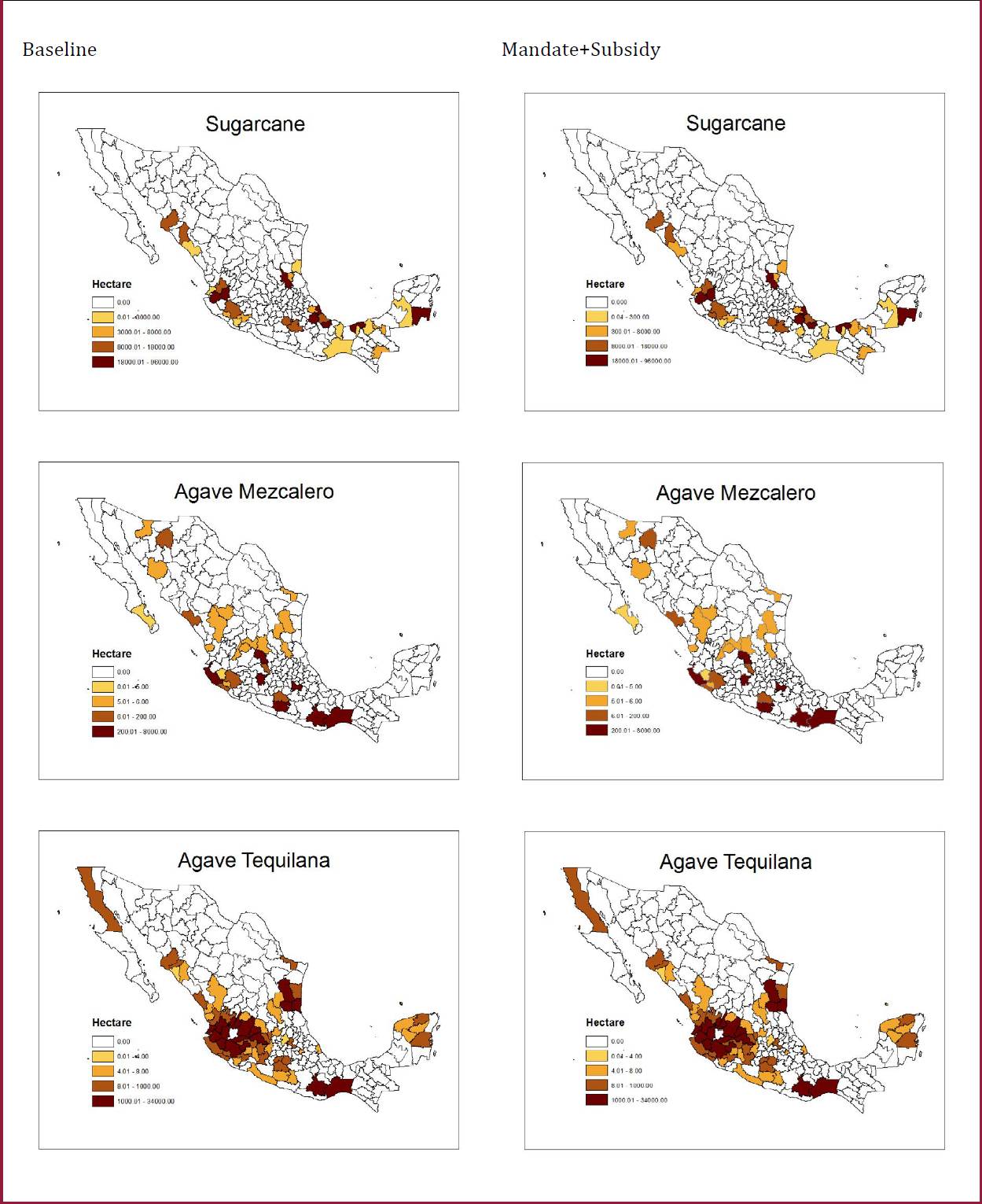
Table 4 Effect of alternatives policies on Ag. Sector in Mexico 2025
| Commidities | Baseline (MMt) | Mandate | Subsidy (% change) | Mand+Subs |
|---|---|---|---|---|
| Demand | ||||
| Bean | 1.792 | 0.04 | 0.00 | 0.00 |
| Sorghum | 4.170 | 0.00 | 0.00 | 0.00 |
| Sugar | 4.375 | -7.01 | 0.00 | -12.57 |
| White corn | 19.200 | 0.00 | 0.00 | -0.05 |
| Mezcal (MMlt) | 1.490 | 0.52 | 0.18 | 0.65 |
| Tequila (MMlt) | 114.208 | -0.04 | 0.00 | -0.04 |
| Supply | ||||
| Bean | 1.649 | 0.05 | 0.00 | 0.00 |
| Sorghum | 4.709 | 0.02 | 0.01 | 0.03 |
| Sugar | 7.724 | -11.70 | 0.00 | -21.00 |
| White corn | 18.599 | 0.00 | 0.00 | -0.16 |
| Mezcal | 2.431 | 0.48 | 0.17 | 0.60 |
| Tequila | 239.571 | -0.05 | 0.00 | -0.04 |
| Price MXN$/ton, MXN$/lt | ||||
| Bean | 6,099.91 | -0.48 | 0.01 | -0.02 |
| Sorghum | 2,882.77 | 0.00 | 0.00 | -0.07 |
| Sugar | 8,627.30 | 24.54 | 0.00 | 44.05 |
| White corn | 3,645.85 | 0.03 | 0.00 | 0.62 |
| Mezcal | 222.02 | -10.07 | -3.48 | -12.60 |
| Tequila | 706.49 | 0.17 | -0.01 | 0.16 |
Finally, Table 5 shows that domestic GHG emissions (in CO2e terms) would decrease only when mandate is in place since ethanol emissions are lower than those from gasoline, when considering all the sectors in the model, CO2e reduction would reach up to 0.8%. This result also is due to more ethanol is imported from the row and less land is required, therefore there are lower domestic emissions. However, this reduction does not compensate economic surplus losses, which are about -0.11% including the environmental gains and fuel and agricultural consumers losses.3 As expected, ethanol producers would get most of the gains from the subsidy since ethanol will be sold either domestically or abroad, in the later case Mexican government would make a transfer of the subsidy to foreign countries, which Mexican consumers would have to pay.
Table 5 Effect of alternatives policies on social welfare and greenhouse gas emissions in Mexico 2025
| Commodities | Baseline (B MXN$) |
Mandate | Subsidy (% change) |
Mand+Subs |
|---|---|---|---|---|
| Agr. producers surplus | 900.72 | 0.876 | -0.001 | 1.116 |
| Agr. consumers surplus | 2,605.43 | -0.378 | 0.000 | -0.668 |
| Fuel producers surplus | 4,142.21 | -1.704 | >100 | >100 |
| Fuel consumers surplus | 10,614.86 | 0.461 | 0.000 | 0.468 |
| Eth. Producers surplus | 0.000 | 0.000 | >100 | >100 |
| Government Revenue | 11.71 | 7.563 | <0 | <0 |
| Total surplus | 11,258.14 | -0.087 | 0.000 | -0.118 |
| GHG emissions (Mt CO2e) | 2,643.74 | -0.763 | 0.000 | -0.791 |
Conclusions and Policy Implications
Mexico has put a good amount of resources on research to develop production of second-generation biofuels, but very little effort to develop a biofuel market for the transportation sector. In this article, a subsidy and a blending mandate policy scenarios are evaluated by using an endogenous-price mathematical programming model. The focus is on ethanol made from agave residues and sugarcane. Agave is one of the largest crop already established with the potential to generate enough biomass for a significant second-generation ethanol production in Mexico. However, the model results have shown that maximum production would be about 2 billion liters when a 15% blending mandate is in place and producers receive a subsidy equivalent to half of the gasoline price. When comparing to international experiences such as the U.S. and Brazil, the amount that Mexico is less than 14% of the production in these countries in the second year of implementing the policies (2004 in Brazil and 2006 in the U.S.). Under the policy scenario of the mandate and subsidy together, sugarcane producers will be able to provide more ethanol than agave producers. The ethanol production from both groups is expected since they are getting the subsidy and making a significant increase in their economic surplus. However anecdotal evidence suggests sugarcane producers are unwilling to bear the fixed costs of setting up production systems because they doubt policies will endure. There has been a surplus of sugarcane in several recent years, but no industrial-scale fermentation or distillation facilities to turn it into ethanol. According to the model results, losses for fuel and agricultural consumers cannot be offset by both ethanol producer and environmental gains. This suggests that some compensating redistribution may be needed if these policies are to be seen as politically sustainable. Likewise, ethanol maximum production is less than 4% of the total projected gasoline demand in the country. Hence it can be concluded that biofuel potential in Mexico is not that high and a significant change in the fuel transportation matrix will require ethanol imports from the U.S. and the rest of the world, meanwhile environmental gains will be low and are far of compensating economic surplus losses.
Important topics that are left out in the present analysis include relaxing some of competitive markets assumptions, for instance, in Mexico sugar mills owners are better described as a oligopoly. Livestock intensification need also to be explored since it is a possibility to release additional land to energy crops. Likewise, other biofuel feedstocks should be considered such as sorghum, residues of corn and sorghum and organic wastes. Other new energy crops that are not developed yet such as jatropha and some alga species deserve special attention too. Other biofuels including biodiesel and biogas have been already study separately, but the integration to this kind of models is left for future research. Regards to biogas, although the gas sector is already included in the model as aggregate supply and demand curves, it will require to model the electricity sector in more detail. All this would require some critical data, in particular costs and yields, which are still subject to high uncertainty. It is worth noticing that most of these biomass and biofuels report substantially lower GHG emission factors. This makes them advanced biofuels and to have a great export potential to the U.S. since second-generation biofuels constitute an important component of the RFS mandates.
It is also worth acknowledging some limitations of this type of models used in this research, so results should be taken with caution. While partial equilibrium models offer a more accurate representation of each sector, they do not account for the interactions with other sectors related to the markets under consideration. Additionally, adjusting certain assumptions such as linearity, rational expectations, and strategic behavior may lead to more accurate results. Modeling them, however, requires information that is sometimes not available, and even if it could be modeled, optimization will often fail to converge to a robust solution.
The purpose of this article is not to send a pessimistic prospective against the development of a domestic ethanol market and it is not either to prescribe a single best choice for the policy instruments considered here. Rather, the analysis aims to call the attention of the industry (e.g., agave, sugarcane, automotive) and the government to start providing incentives and commands to both the demand and the supply sides since now. The empirical results presented here can provide useful guidance for the government and the industry. For instance, these results could guide domestic biofuel industry to compensate a reduction in the world supply due to changes in trade or environmental policies from other countries. Since ethanol production would be low under the policies in consideration, the model can become a useful tool to assess future policies that aims to develop a domestic biofuel market such as international trade tariffs, tax policies, law enforcement by regulatory agencies, or environmental policies.

