text new page (beta)
 English (pdf)
 Article in xml format
 Article references
 Send this article by e-mail
 Cited by SciELO
  Similars in
SciELO
Similars in
SciELO 
 Permalink
INTRODUCTION
This paper analyzes the interaction between global and local information and its effect on individual choices. In this paper, information refers to the proportion or number of agents in a social context who have previously made one choice or another. An agent processes such information and, along with other influencing factors, determines which action to choose from a set of options. In this setting information is necessarily transmitted through the individuals’ social networks. It is reasonable to suppose that most of the time agents only have access to local information, i.e., information that is constrained to the closest social links —neighborhood, family, friends, co-workers—. But, from time to time agents can also have access to global information, that is, information that represents what is happening in society as a whole. The purpose of this essay is to study both local and global information at the same time and evaluate their effects on individual binary choices and aggregate behavior. The practical implication of this study is to have an understanding of the effects that mechanisms producing global information —like polls, economic reports and media broadcasting— can have on a population that is also engaged in local dynamics.
Both global and local interactions are often found in many social dynamics. For example, the incidence of crime can be very sensitive not only to neighborhood levels of criminality, but also to community levels ( Glaeser and Scheinkman 2001 ); the investment decisions of a firm can depend on both monetary policy —global signal— and investment decisions of the firms located in a specific spatial and industrial cluster ( Albin 1998 ); individuals can make inflation expections using information from «experts» who have access to the media and from conversations with their neighbors or friends ( Carroll 2003 ); and pre-electoral polls —global information— can influence individual preferences, which themselves are influenced by local dynamics from interactions with friends, coworkers or neighbors.
In this essay, it is argued that the study of the interaction between local and global information produces new insights into understanding social dynamics, even when binary choice and simple neighborhood structures —like von Neumann— are considered. This paper is structured as follows. In section 2, a brief theoretical background is presented. In section 3, the model of individual decision-making is described. Section 4 provides the main results of the model when both local and global information are simultaneously considered. And the paper ends with a concluding remarks section.
THEORETICAL BACKGROUND
Schelling (1978) is the classic text in which the fundamental aspects of the social phenomena studied in this essay are discussed. For example, his famous neighborhood model of residential segregation ( Schelling 1978, Chapter 4 ) can be understood as either a model of local information —self-forming neighborhood model— or global information —bounded-neighborhood model—. Likewise, threshold models of collective behavior a la Granovetter (1978 , 1983 , 1988) , in which choices are seen to depend on the proportion or numbers in some reference group, are formulations that model global information. In recent years, new literature on social interaction in economics, most of it associated with the Santa Fe research program ( Arthur, Durlauf, and Lane 1997 ), has produced theoretical studies on social phenomena that take global and local information into account. For example, by incorporating well-established models in statistical mechanics, Brock and Durlauf (2001 , 2003) propose a baseline model of socioeconomic behavior with interdependencies that describe the properties of and individual discrete choice specification subject to global information. These approaches are sometimes called random field or «mean field» —a terminology employed in studies of magnetism— because the interactions of a large number of microunits —agents— are subject to aggregate effects.1
Likewise, along the same lines as the global interaction theoretical track of thought, a great variety of local interaction models have also been proposed. In such models, agents interact only with a subset of other agents in the population —e.g., neighbors—. Models from the physical sciences like the Ising model, the voter model and contact process have influenced analytical developments in evolutionary game theory, considering low rational individuals under local interaction dynamics ( Blume 1993 ). Along the lines of the computational approach, using agent-based models in social science has become a very important methodology for analyzing social interactions and long-run dynamics under conditions of agent heterogeneity, adaptation, different rules of behavior and bounded rationality ( Epstein and Axtell 1996 ). The methodology has also been used to study issues related to local information dynamics ( Epstein 2001 ).
The approach followed in this paper is computational, but also used are probabilistic models from the social interaction literature ( Brock and Durlauf 2001 ) that adapt standard discrete choice models (like McFadden’s conditional logit model, 1974) to the particular situation of social interdependence. We use a dynamic framework of individual decision- making that can be interpreted under the assumption that agents have «naive or myopic expectations» because they are using current average choice as the basis for expectation formation (similar use can be found in Brock and Hommes 1997 , Young 1998 ). Because the model is studied under conditions of agent heterogeneity and the agents are interacting either locally —with their neighbors— or globally, we preferred to resort to a computational approach that resembles agent-based model practices. The methodology not only allows us to identify long-run stationary distributions —like those predicted by theory in simple cases—, but is also flexible enough to allow for the collection of data from dynamics that otherwise would be difficult to gather.
THE MODEL OF DECISION
Agent i chooses action ω —from a Ω discrete set choice— which reports a «utility» to her. An underlying latent variable Y* exists such that it denotes the indirect «utility» associated to action ω . The underlying utility depends on:
where h is a private incentive that can be a function of sex, education, etc., S is a social interaction term that reflects the behavior of the agents other than i in choosing ω —in a reference group—, and ε is a random variable —which can register unobservable variables that affect agent i action—. A particular specialization of (1) reports the following payoff function of agent i in choosing action ω:
where
Equation (2) is a case of social influence with proportional spillover effects in where agents wish to match the average decision of the community; likewise, the model introduces J which is a parameter of social strength. This specification is similar to the one analyzed in Brock and Durlauf (2001 , 2003) .2
Now, by invoking standard behavioral rules in economics, it must be expected that equation (2) responds to a rational decision such that Y* (ωi,k) = Max(Y* (ωi,1), Y* (ωi,2)...Y* (ωi,k)), where k is the total number of choices.3 It can be shown ( McFadden 1974 , Maddala 1994 ) that if ε(ωi) are i.i.d. with the type I extreme-value whose cumulative distribution function is:
a standard multinomial logit approach can instrument a probability for agent i in choosing ω such that its payoff is maximal among all the payoffs available to the agent:
The model produces a common parameter β , which controls the extent to which the random term is important. If β → ∞ , the random term is unimportant and it means it is highly likely that the «best action» is taken by the agent, while β close to zero implies that choice decision is mostly random. As indicated in equation (2), the model has a parameter J that indicates the intensity to conform to the behavior of others; therefore, the probabilistic model in (4) has a compound parameter βJ that controls the social interaction effect.
It is important to remark that equation (4) implies that the effect of the social interaction term is endogenous. That is, there are interdependencies in choices among the members of the community, and that makes the social interaction effect reflexive —anagent’s behavior influences the other agents just as she is influenced by them—4 . This is what makes the model different from a standard application of discrete choice models.
Suppose that agents are facing only two options: +1 and -1. Consequently, the decision framework, at time t, can be reduced to a familiar logit model of the form:
conversely,
Note that in this formulation, agent i has perfect knowledge of the
average choice
about a(t) ; in this sense, equation (5) would imply that agent i has «perfect foresight»: ai(t) = a(t) . That is, under the symmetric conditions of equation (5), it would be necessary to impose «rational expectations» such that each agent i has a common expected value of the average choice.
In contrast, we think that is more appropriate to model (5) in an adaptive way such that agents «expect» the average choice at time t+1 to be the same as it is in the present period t: ai (t+1) = a(t). Under this formulation, it is possible to take into account any possible mechanism available to agents that can aggregate information at time t (or t-1). Therefore, equation (5) is transformed in:
The latter types of probabilistic models have been analyzed in physics —random fields—, and they have been incorporated into economics to explain individual choice.5 A final remark related to this point indicates that equations (5) and (6) imply a «non-cooperative» behavior of agents because no communication or coordination exists between them —agents are only incorporating information of what the others are doing.
FRAMEWORK OF SIMULATION
Analytical results have been provided when agents are facing decisions under conditions of choice expressed in equation (5) in a context of static global interaction in where agents interact symmetrically ( Brock and Durlauf 2001 , 2003 ). Interestingly, analytical results have been also proposed in dynamic local interaction settings ( Young 1998 ). The key insight in this approach is to have a spatial model of choice in where agents are enrolled in an adaptive learning process —like equation 6—, and it is possible to calculate the long-run probability of states —i.e., proportions of agents in choosing an action—. Such long-run probabilities result in a stationary distribution that is known in physics literature on interacting particles as Gibbs Distribution.
Nevertheless, when private incentives are nonconstant —or heterogeneous— (h’s) among agents in equation (5), general propositions tend to be difficult to establish for the global interaction case ( Brock and Durlauf 2003: 12 ). For extension, the same happens in the local interaction case when heterogeneity in private incentives is taken into account —that is, when idiosyncratic payoffs are not zero—. If in addition a mixed model of global and local interaction is considered, it seems to be appropriate to resort in principle to computational simulations to understand the properties in such systems. This is the methodological approach that we will follow.
The basic rules of the simulations are the following: 399 agents (N) are dispersed in a 21 X 19 wrapped two-dimensional lattice. Each cell of the lattice corresponds to one agent and she is at the center of the cell, such that the nearest neighbors of agent i are located within Euclidian distance 1 from agent i. It is assumed that each agent i has 4 nearest neighbors —which is equivalent to the von Neumann neighborhood—. The initial configuration of states (+1, -1) is random such that the sum of all initial agent choices is close to zero. Private incentives (hi) are randomly assigned at the beginning to each agent, according to a normal distribution —most of the simulations treat the mean of the distribution as fixed (and equal to zero) and only the standard deviation is controlled—. The private incentives remain fixed through the dynamics. An agent i updates her choice at random times governed by a Poisson arrival such that on average each agent updates once per unit of time —that assumes a λ = 1 such that, the probability of an agent to update is pi = 1/N —. When an agent i updates, she has a probability δ of choosing an action +1 or -1 with global information and, a probability 1 - δ of choosing an action +1 or -1 with local information.6 If an agent updates with global information, she has a probability of choosing an action +1 given by equation (6); otherwise, she is updating with local information with a probability given by (7):
where
Note that in the simulations it is assumed that any agent that updates with global information has access to actual numbers of the system at that moment.7
In the next sections, the results of the simulations are presented.8 In the appendix, we present the simulation interface in NETLOGO 2.02. of one typical realization.
GLOBAL AND LOCAL INFORMATION EFFECTS
SELF-FULFILLING PROPHECIES
When agents are updating their choices based only on local information —see equation (7)— with private incentives (h’s) equal to zero and when β is high enough, the system tends to produce nontrivial outcomes. To illustrate the latter, consider Figure A that shows the long-run distribution of the average choice when β = 100 . The results indicate that even though the distribution tends to be skewed and concentrated in the extremes, there is space for nontrivial outcomes; note for example that the distribution «jumps» a little bit in the center. The important element to highlight from Figure A is how a simple framework of «local imitation» —where private incentives are not considered at all— is able to produce nontrivial multiple equilibrium as «stochastically stable states» or to generate long «transient configurations» —a la cellular automata— –broken ergodicity.9
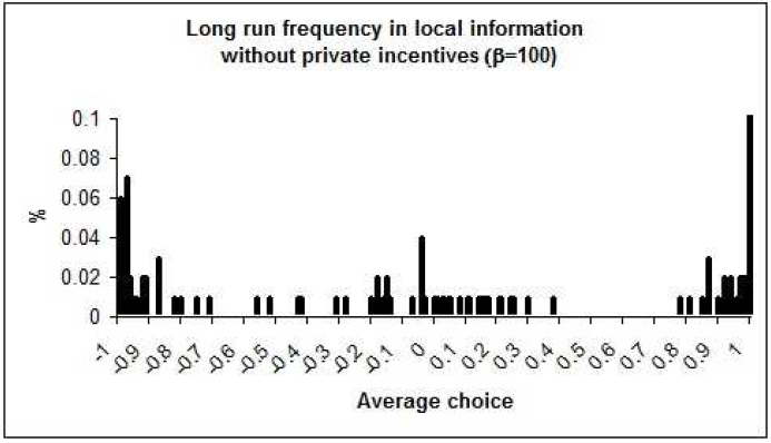
Figure A. Long-run distribution of the average choice in a local information setting without private incentives and with a parameter β = 100
100 replicates are run and the average choice is calculated during a period of 250 time- steps. A warming up period of 100 time-steps is considered to calculate the average choice.
What happens if both local and global interactions are considered in the dynamics —under conditions of a von Neumann neighborhood—? It can be shown that at least for the case of homogeneous private incentives, global information percolates through the network. It does so in such a way that the long-run frequency distribution will exhibit only extreme outcomes once the parameter β —see equation (6)— is high and enough agents using global information in their updating of decisions are considered in the dynamics —two peaks type distributions.
As an example, consider that when an agent reconsiders the choice she made, the probability of her updating her choice using global information is δ ≈ 4 / 399 . That is, approximately 1% of agents adjust globally —with equation (6)—, while the other 99% of agents adjust locally —with equation (7)— for each time period. In each period, new «global agents» —those who reconsider their decision using global information— are randomly chosen; we can call them «random global agents». The rest of the conditions of the simulation remain such that h’s are set to zero.
The basic result of the simulations indicates that consensus outcomes are always produced under these conditions. If we conceive of those «random global agents» —note that they are not fixed— as people who gather information from polls or media from time- to-time, then these global actors either accelerate extreme outcomes or —more interestingly— make the coexistence of choices improbable in the long run. Under these circumstances, local and global interaction dynamics do not differ from each other in the long run.10 If we consider Figure A again, the long distribution under the influence of «random global agents» would be one that concentrates equilibrium outcomes only in the extremes of the distribution.
It is not difficult to see that the latter result does not depend on the network structure or connectedness of the network.11 In other words, global information presented in the model analyzed can arrive to either poorly connected people —who have an opportunity to break their local informative trap— or highly connected people —who can activate cascades—, but this does not affect the long-run equilibrium outcome under conditions of homogeneous private incentives.
It is important to note that it is not necessary to have «random global agents» to break the local clusters generated by local interactions. A simple diversity of opinions among these agents —or a random choice— might also move the system towards extreme outcomes, regardless of the «network structure». Likewise, different «visions» do not strictly indicate different «networks», because the connection between agents is not necessarily symmetric. Nevertheless, working with real «networks» should not alter the basic results mentioned so far.
Self-fulfilling outcomes are interesting theoretically, but otherwise are of little practical importance because social phenomena rarely exhibit extreme outcomes. In contrast, relevant cases are those when reversals appear in the social dynamics because oscillations rather than convergent extreme outcomes are the generic features that social interactions display in real life. We will analyze these cases in the following subsections.
REVERSALS AND CASCADE EFFECTS: FROM LOCAL INFORMATION TO GLOBAL INFORMATION
In the argument that follows, we study the possibility of producing reversals and cascade effects generated by global information, affecting steady states produced by purely local interactions. The dynamics under study begin under conditions of local interaction ( δ = 0 ) and, once the system stabilizes —i.e., reaches the stationary distribution—, global interaction behavior is introduced ( δ ≠ 0 ) into the dynamics in order to evaluate whether or not the «stationary distribution» is affected by global information. The cascade effect is evaluated with respect to changes in the aggregate choice decision. A reversal is considered if a positive average choice in the steady state generated by global interaction is smaller than the average choice in the steady state produced by only local interaction. When the final average choice is negative, it works in the opposite manner.12
Now, heterogeneous private incentives (h(i)) are introduced in the simulations: h’s are randomly assigned from a normal distribution with a mean of zero, and different standard deviations are considered in the simulations. It can be shown that when β → ∞ the system produces nontrivial stationary distributions; so, we decided to choose β = 100 to run the simulations in order to guarantee that condition. This also has another important implication in the sense that the «random utility» factor is unimportant when it allows us to evaluate possibly large variations in the system because of factors other than randomness.
In the simulations, each replicate starts with δ = 0 —i.e. pure local interaction— and it is allowed to run for 200 periods of time, at period-time 200, δ ≠ 0 , such that global random agents enter in play and the system runs for 200 additional periods of time.13
First the scenario in which everyone is converted to a global agent was analyzed; that is, at time 200, δ = 1. This scenario would be equivalent to a situation where a poll or an economic report —that reports or estimates the actual majority of the whole community— is published and everyone adjusts their decisions based on this global information.
Fifty replications for each condition of the simulation were run14 and V’s —visions— among agents were kept constant and equal to 1, such that a von Neumann neighborhood of local interaction was simulated. However, one simulation was run with heterogeneous visions to see the possible effects of the «social network». As stated earlier, heterogeneous h’s with different levels of dispersion are also considered in the analysis. Table 1 summarizes the results.
Table 1. Reversals and size of cascades: from local information to global information
| Dispersion in Private Incentives/mean is zero | 0 | 0.1 | 0.5 | 1 | 1 |
| Neighborhood | von Neumann | von Neumann | von Neumann | von Neumann | Heterogeneous |
| Reversals rate | 0 | 0.02 | 0.06 | 0.26 | 0.52 |
| First period average | 0.011 | 0.050 | 0.008 | -0.005 | -0.022 |
| First period average (absolute) | 0.691 | 0.227 | 0.136 | 0.077 | 0.102 |
| Increase average (absolute) | 0.309 | 0.771 | 0.806 | 0.138 | 0.114 |
| Final average (absolute) | 0.999 | 0.998 | 0.941 | 0.216 | 0.217 |
The first interesting result to mention from Table 1 is that global information does not always reinforce the decision that is held by the majority, which happens when “private incentives” are homogenous among agents. When the standard deviations in private incentives are close to zero, the reversal rate —number of reversals over total runs— is almost zero. However, the rate grows positively in a nonlinear manner with higher levels of dispersion in «private incentives»15 . For example, with dispersion equal to one —fourth column—, the probability of a reversal is ¼. More drastically, when the neighborhood structure is heterogeneous16 and dispersion is high —last column—, there is a fifty-fifty chance of a reversal.
Reversals take place because, for some agents, global information reports to them a smaller proportion of the majority’s opinion than the one they obtain with local information, and this change of information can be enough, given their «private incentives» —which must be opposite to the signal indicated by the majority—, to reduce their propensity of going with the majority. This can be an interesting rationale for the so-called underdog effects.
It can be seen from Table 1 —see last row— that consensuses —or extreme outcomes— are observed when the standard deviation in «private incentives» is between 0 and 0.5 —note that the final average is almost 1, implying that everyone is «coordinated» on one choice—. The average size of the «cascade» increases with higher dispersion in private incentives. Nevertheless, cascade sizes sharply decrease —and consensus outcomes are no longer dominant— when dispersion in private incentives is set to 1 —see fifth column of Table 1 —. It seems there is a threshold in the dispersion of private incentives that makes the system change qualitatively in terms of its dynamics. When the system is suddenly subject to global information, nontrivial stationary distributions appear, cascades become less predictable and reversals emerge. The role of private incentives in affecting the stationary distribution in these kinds of dynamics is also found in the Bayesian literature of global interaction ( Orléan 1995 ).
The last column of Table 1 shows the results of the simulations with heterogeneous vision in agents.17 The results do not differ substantially from those exhibited in the von Neumann case in relation to cascade sizes and nontrivial stationary distributions. Nonetheless, note how the probability of achieving a reversal increases up to ½.
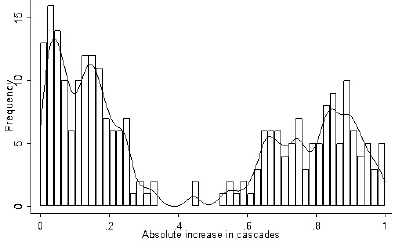
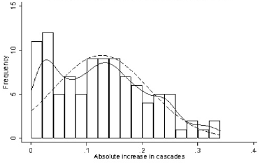
The cascade sizes exhibit interesting distributions. Figure 1 displays two histograms using a bin equal to 0.02 —that indicates the absolute value of the % of increase—. The distribution of Figure 1.A contains cascades with different levels of dispersion in private incentives —with a mean of zero—, while the distribution of Figure 1.B only considers cascades whose standard deviation is equal to one —with a mean of zero—. Both histograms in Figure 1 also display the Gaussian Kernel density. The histogram on the left is clearly bimodal and it simply confirms what the data in Table 1 indicates when different levels of dispersion in private incentives are considered. The distribution of Figure 1.A is skewed to the right when the increase in cascade is relatively small and it is skewed to the left when the increase in cascade is high. The skewed right distribution in Figure 1.B is associated to high levels of dispersion in private incentives; to see this, the distribution —see Figure 1.B — contains only cascades where private incentives have a standard deviation equal to one. Note that the distribution ( Figure 1.B ) is also skewed to the right. The histograms suggest that a type of exponential distribution might describe the cascade sizes when the system moves from local interaction to global interaction: a «negative exponential» is associated to high levels of agent heterogeneity in private incentives, while a «positive exponential» emerges with low levels of agent heterogeneity. Later on in this paper the distribution of cascades —and their «exponential» shape— under local-global interaction dynamics will be discussed in more detail.
The data indicates that normal distributions are not appropriate for describing the size of cascades produced by the system when there is a change from local interaction equilibrium to global interaction equilibrium. A practical implication of this finding is related to the potential —otherwise underestimated— of pre-electoral polls or economic reports to activate a large avalanche of choice/opinion changes in population dynamics.
Figure 1. Histograms of cascade sizes with heterogeneous private incentives when the system changes from local to global interaction
Figure 1.A considers different levels of dispersion in private incentives with a mean of zero, and it contains 250 replicates —see summary of the data in Table 1 —. Absolute increase in cascades is calculated in the steady states. The bin width used in the histogram is 0.02. The continuous solid curve is the normal —Gaussian— Kernel density with bandwidth 0.02 —the same as that used in the histogram—.
Figure 1.B only considers 100 replicates with private incentives whose mean is zero and standard deviation equal to one, and the data contains 50 replicates. The continuous solid curve in Figure 1.B is the normal —Gaussian— Kernel density with bandwidth 0.02 —the same as that used in the histogram—. The dashed curve is the normal density.
GLOBAL INFORMATION AS AN UNSTABLE MECHANISM
Now, what happens if not all agents but only a fraction of them have access to global information? To respond to this question, we present information from 20 replicates, each of which consists of 600 time steps, with the following conditions: β = 100 , heterogeneous «private incentives» with a mean of zero and a standard deviation of 1, a von Neumann neighborhood structure and random initial conditions with aggregate choice value close to zero. In each replicate, the simulation begins with zero «random global agents» (i.e., δ = 0 ) and, when the simulation reaches time-period 200, all agents when updating their choice start to adjust globally (i.e., δ = 1); and finally, at time 400, approximately 50% of agents start to adjust globally each period while the rest continue to gather only local information (i.e., δ = .5 ). A warming up period of 50 time steps —after δ changes— is considered when calculating statistics. Here we want to remind the reader that the social strength parameter J has been set to one in all simulations such that the compound social interaction parameter βJ is controlled only by β to simplify the simulations.
The results of the simulations indicate that the time series are pretty stable in the extreme cases when agents adjust only with either local information or global information, nevertheless the series become highly perturbed with 50% of random global agents. To illustrate this, Figure 2 presents the standard deviation of the choice value observed in each replicate for the three cases analyzed. As we can observe, the variance in the extreme cases is in both cases similar and quite low —there the system is in the stable equilibrium—, but note how the standard deviation is much higher when only 50% of agents are adjusting with global information.
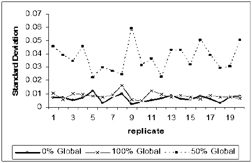
Each series indicates the standard deviation in the aggregate choice that a percentage of active random global agents produces —the rest of the agents behave locally—. Each replicate consists of 600 time-periods.
How much is the stability of the system depending on the actual numbers of random global agents? To see this, simulations now consider different δ’s in the same replicate; specifically, after each 200 time-periods, the number of random global agents is increased by 10 percent points. Each replicate starts from zero random global agents (i.e., δ = 0 ) and it ends with 100% of random global agents (i.e., δ = 1). Figure 3 displays the time series of the average aggregate choice value for an interesting and particular realization.
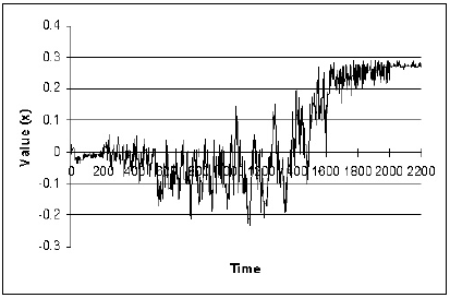
Figure 3 . Time series of the average aggregate choice subject to different levels of global information —a particular realization—. Each 200 time-steps, the percentage of agents that update with global information increases by 10 points; the series starts with zero global agents and it ends with 100% of them.
Figure 4 . Average choice in different intervals of global information —a particular realization—. The data is the same as that used in Figure 3 ; now the average choice value and the standard deviation in the interval are calculated —the upper-low bands are calculated using a 95% confidence interval.
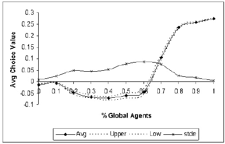
It is clear from Figure 3 that the extremes are the more stable periods —where everyone is adjusting either locally or globally—, while the middle periods are the more unstable. In this particular realization, dispersion in the aggregate choice value increases when more random global agents are active; it is important to note, however, that bigger oscillations in the series do not seem to change the basin of attraction —which is close to zero— until the time series crosses 1,400 periods —where 50% of random global agents are active—. After that point the basin of attraction moves upward quickly until the system is stabilized again during the final section of the curve. The system suddenly displays a «hysteresis phenomenon» associated to a corridor of drastic changes —the steepest section of the series—, suggesting the system is experiencing a «phase transition» from local interaction equilibrium to global interaction equilibrium. These changes are best appreciated by taking the average value per 200 time-periods; Figure 4 displays the results —the standard deviation is also considered in the figure; also a warming up period of 10 steps is used to calculate the average—. First, note that the standard deviation is maximal with around 50% of random global agents. It is interesting to see that in this particular realization «global information» does not reinforce the «optimal majority» until the system gets more than 60% of global agents; that is, the system gets trapped in a lower equilibrium and even reinforces it when random global agents are not so many, and it seems to escape from that equilibrium when the number of global agents is only high —greater than 50%.18
This typical realization illustrates clearly how global information does not produce clear bandwagon effects as is the case with homogeneous private incentives. Global and local information interact in such a way that the system is not only perturbed —generating oscillations— but it can also be trapped in a basin of attraction if a big number of global agents are not operating. A big push of random global agents is required in order to move the system to the upper equilibrium.
CASCADES AND DIVERSITY IN GLOBAL INFORMATION
Is the type of behavior described in the last section a common feature in all simulations?
In order to look at this, we make the different time series produced by the different replicates comparable by averaging the size of their cascades. The size of a cascade is defined as how much the average choice value increases —or diminishes— when the system starts to be perturbed with global information. The simulation consists of 40 replicates, and as in the case of the latter simulation, the number of global agents is increased 10 points each time the system performs 200 time-steps until all agents are updating with global information (i.e.,δ = 1). The average size of cascades is calculated using the absolute increase in percentage points —absolute values are used because reversals are possible.
Figure 5 summarizes the results. Each point in the dark curve relates to the percentage of global agents (x-axis) with the cumulative increase of cascade sizes (y- axis);19 for example, 50% of global agents produce 80% of the total increase in the aggregate choice value. In this way, the dark curve can be seen as a Lorenz curve where the 45o line would represent the perfect equality between cascade increase and global agents —i.e., cascade increases are proportional to the percentage of global agents—. The small dashed curve —that looks like a quadratic function of concave form— shows the average standard deviation in the aggregate choice value in the series —a scaling factor of 20 is used to facilitate comparisons—. Note that in the extreme cases —0 and 100 of global agents— the dashed curve dispersion is minimal, indicating the system is stable at the extreme points.20 Also note that minimal dispersion coincides with the intersection of the 45o line and the dark curve; as we observed earlier with the particular realization in the last subsection 4.3, these points represent the system’s two generic equilibria: the lower left corner of the figure represents local interaction equilibrium while global interaction equilibrium is at coordinate.
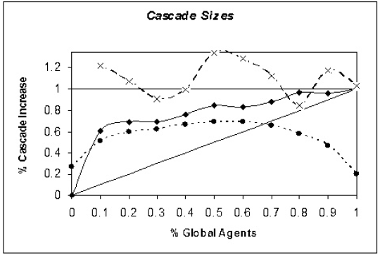
Figure 5. Cascade sizes produced with different levels of global information and heterogeneous private incentives. Dark curve with small dot indicates cumulative cascade increase; dash curve with small dot corresponds to the standard deviation of cascades (with scaling factor of 20); dash curve with cross dot shows the coefficient of variation for cascades. Each point represents an average of 40 replicates. βJ = 100 , the mean of h’s is zero and their standard deviation is 1. A total of 399 agents are dispersed in a wrapped two dimensional lattice.
Figure 5. also displays the coefficient of variation for cascades —see large dashed curve with cross dot—; this curve has an interesting oscillating behavior indicating that high variations of cascades —i.e., the possibility of large events— are more likely to occur either close to the extreme cases or in the middle —50% global agents.
Figure 5. illustrates how the system gets a «big initial push» on average with only 10% of random global agents —60% of the total increase is explained by the initial push—. Also note that the system gets easily perturbed from the beginning as well: not only does the standard deviation in the average choice increase, but also the coefficient of variation for cascades is at a local maximum. Another interesting feature of Figure 5 is that the dark curve suggests that interval periods with low cascade activity follow periods of relatively higher activity. This can be an indication that the system displays some «phase transitions» where the average choice values increase drastically as suggested above when presenting a particular realization.
Figure 5 also shows how the standard deviation of the aggregate choice value grows rapidly with just 10% of global agents, but then grows at a much slower rate until it reaches a maximum in the middle. The system becomes highly perturbed with 50% of random global agents. These high levels of dispersion indicate the series is oscillating drastically —in nontrivial way— around a gravitational point —which is indicated by the dark curve—. The interesting point here is that the system can even be «touching» the system’s two extreme equilibria; in other words «global information» at this point does not give a clear signal to agents to «coordinate» in one of the equilibria —local or global—. In real life, extreme cases —local or global— are not expected, but rather a combination of them; consequently, the model would predict that the average choice is unlikely to be fixed or stabilized —by the way, this is a stylized fact in opinion dynamics—. Heterogeneity in the private incentives is the clue here to see why global information —in combination with local information— produces such dynamics. If private incentives are homogenous, the latter situation is reduced to an extreme case of trivial full cascades. Therefore, greater heterogeneity in private incentives makes the system more perturbed and unstable —this is the cost of having greater plurality in agents.
Something else interesting to note in Figure 5 is that the large dashed curve of the coefficient of variation has an up-and-down behavior indicating that larger variations in cascade sizes are more likely to happen at the extremes —with few or many global agents— or at the middle —with half of the global agents—. This suggests that large cascade events do not necessarily depend on the number of global agents. The distribution of cascades along the spectrum of active random global agents is displayed in Figure 6 , and the bin width considered in the histogram is 0.025 —which represents 2.5 percentage points of cascade increase—. The mean of the cascade size is 0.18 —standard deviation equal to 0.24.
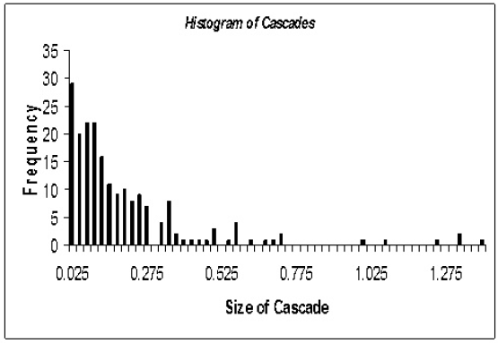
Figure 6 : Histogram of cascades with diversity in the levels of global-local information. The bin (x-axis) represents 2.5 percentage points of cascade increase. There are 200 observations, each one associated to different levels of random global agents. Each observation indicates the average size of cascade —in percentage points— obtained by the system when it is injected with random global agents.
Figure 7 . Tail cumulative frequency of cascade size in semi-log space. 194 observations are considered from data in Figure 6 —six observations whose value exceeds 0.9 were excluded—. The solid line represents OLS regression estimation.
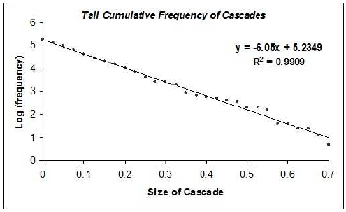
The distribution of frequencies in Figure 6 exhibits an exponential decay. In order to see this, Figure 7 displays the tail cumulative frequency of the data from Figure 6 in semi-log space.21 The distribution of the transformed data is linear; OLS regression yields a R2 = 0.99 and a slope of –6.05 (SE=0.111) and intercept of 5.235 (SE=0.045). The regression results suggest that the distribution of cascade size coincides with a negative exponential distribution.22
Note that exponential decay is obtained in the distribution when diverse levels of global agents are considered. We saw earlier that when the system jumps from zero global agents to 100% global agents, the distribution of cascades is symmetric but with fat tails —see Figure 1 —. Now, when diverse levels of random global agents are considered —see Figures 6 and 7 —, the distribution of cascades suggests an exponential law. This type of distribution is ubiquitous in physics for characterizing a conserved variable like energy; likewise, exponential distributions are used to characterize failure rates —mainly in electrical and mechanical systems— with a «lack of memory» property. This would mean that the size of cascades is subject to a constant growth rate that is independent of size; and this implies that the probability of a cascade occurring in a specific size interval is the same regardless of the starting point of the interval size. In other words, in order to calculate the probability of the final size of a cascade in a specific interval size, the size of the cascade that the system may be experiencing before it reaches equilibrium does not matter.
Watts (2002) has proposed that binary choice models can produce cascades with power law distributions —and bimodal distributions, too—. He emphasizes the roles of thresholds and network heterogeneity to arrive at such outcomes. Here instead, we find exponential distributions of cascades under a rationale that emphasizes local-global information and heterogeneous private incentives when different levels of agents subject to global information are taken into account.
CONCLUDING REMARKS
In this essay, the case is presented that some of the common theoretical results derived by scholars when studying issues related to the effects of information dynamics on individual choice can be understood well by studying the interaction between the global and local information to which society is exposed. This is a novel approach because global and local interaction dynamics tend to be studied separately.
What is very uncommonly seen in the discussion of social interactions is that heterogeneity of agents —private incentives— can sometimes be in agreement with global information but in conflict with local information —or vice versa—. In other words, it is possible that heterogeneous private incentives can reinforce the actual majority in the community but weaken the local majority —of their local network—. This is a very important possibility to highlight because, in real life, people frequently receive diverse streams of informational data: sometimes information comes from their social network —friends, family, and neighbors—, and at other times, the information might represent the entire community —polls, media and experts—. What the framework of analysis presented here indicates is that such heterogeneity in information could be enough to produce nontrivial dynamics in the aggregate choice.
In today’s world, more people have access to global information —in the form of polls, media or economic reports— that forecast future events. Thus, how can this situation —that can potentially generate self-fulfilling prophecies— be reconciled with the possibility of maintaining not only diversity in choices but also continuous changing of choices? One way to address this, as observed in economic literature, is by internalizing the social effect in a rational individual framework in which social influence is counterbalanced by the agent’s self interest component. By increasing the private incentive component, multiple equilibria —and diversity of choices— are generated even when there is a strong presence of group effects. However, this approach assumes that the data stream of information comes from only one source —either global or local.
Another way to analyze this situation is by using this essay’s hypothesis. That is, individuals continue to behave locally, but from time to time they have access to global information. By considering this simple heterogeneity in the data stream of information, it is also possible to derive results characterized by opinion dynamics, such as tipping points, and abrupt changes in the aggregate and punctuated equilibria.
By studying global and local dynamics of information, this paper also suggests that both bottom-up and top-down mechanisms of interaction must be considered in the study of social behavior. This line of reasoning is more in accordance with what the literature in Institutional Economics has suggested about collective learning and the emergence of institutions ( Mantzavinos, North, and Shariq 2003 ). One way to perceive this point is by considering that «institutions», by aggregating relevant information, can reduce uncertainty —or reduce computational costs— in individual decisions. However, society has informal institutions and formal institutions. One way to understand this is that local information dynamics can be a proxy of informal institutions, while global information dynamics can be an expression of formal institutions. The interaction between formal and informal channels of information can stabilize the system, but can also sometimes make it highly unstable and fragile.
This paper has made strong assumptions about the way global information arrives to agents. In particular, the model analyzed here assumes that every agent has the same likelihood to receive global information, and clearly this is not the case in real life. Also, it was assumed that the intensity parameter of social strength is the same among diverse groups. These issues, along with others such as more appropriate topologies of local interaction and multinomial choices, should be studied in future research. Likewise, another natural step to follow would be to devise some econometrics —implementing standard discrete choice models— or to design an empirical computational approach.