


 nueva página del texto (beta)
 Inglés (pdf)
 Artículo en XML
 Referencias del artículo
 Enviar artículo por email
 Citado por SciELO
  Similares en
SciELO
Similares en
SciELO 
 Permalink
PACS: 41.20.Jb.
1. Introduction
The introductory examples of electromagnetic radiation, in the advanced undergraduate and graduate levels, are commonly those of the Hertz electric and magnetic point-dipole sources with a harmonic time variation; in addition the study of the electromagnetic radiation in resonant cavities is presented separately 1,2,3,4,5,6,7,8,9,10,11. Our experience with the multipole expansions of the electrostatic and magnetostatic fields 12, and of the electromagnetic fields 13 and of their respective sources distributed on a spherical surface, shows the existence of complete and exact solutions inside and outside such a boundary surface, for each multipole component. In this contribution, we construct the electromagnetic radiation solutions for the finite electric and magnetic dipole sources, applicable for both antennas and resonant cavity modes.
In Sec. 2, the magnetic dipole case is analyzed first because it is didactically simpler. In fact, it involves a surface current with a sine of the polar angle distribution along parallel circles. Then, the vector potential and the electric intensity inherit the alternating time variation, the dipolarity and parallel-circle field lines of their source; additionally, they share the same radial dependence in terms of spherical Bessel functions of order 1: ordinary ones inside and of Hankel type outside, and with coefficients involving the other function at the radius of the boundary surface guaranteeing their continuity there. The magnetic induction field is evaluated as the rotational of the vector potential, with radial components continuous at the boundary surface, and polar angle tangential components with a discontinuity connected with the source current by Ampere’s law.
On the other hand, in Sec. 3 the electric dipole source consists of a surface charge with a cosine of the polar angle distribution, and a surface current with a sine of the polar angle distribution along the meridian half-circles on the boundary spherical surface; both distributions are connected by the continuity equation. In this case the solutions are constructed first for the magnetic induction from the Helmholtz equation with its rotational of the current source. The latter shares the same dipolarity as the original current and its field lines are parallel circles. The solutions are evaluated as the integrals of this source with the outgoing-wave Green function in its multipole expansion form: only the dipole term contributes, the parallel circle field lines and the radial inner and outer spherical Bessel functions are also inherited, with coefficients involving the derivative of the radial coordinate times the other Bessel function at the radius of the spherical boundary surface. The magnetic induction field is discontinuous at the spherical boundary, and their discontinuity leads to the meridian current as demanded by Ampere’s law. Next, the electric intensity is evaluated via the Maxwell connection as the rotational of the magnetic induction, exhibiting field lines in meridian planes with discontinuous radial components at the spherical boundary surface, connected with the charge distribution by Gauss’s law, and continuous tangential components at the same boundary.
In both sections, the exact solutions lead to analytical forms for the field lines in the meridian planes of the magnetic induction and the electric intensity, respectively, inside and outside; they turn out to share the same shape. Inside they have opposite directions, reflecting the nature of their respective sources; and for the same reason, their continuities and discontinuities at the boundary surface are different and complementary. The outer solutions can be analyzed in the very near quasi-static and in the very far radiation limits, connecting with the standard analysis in the books. An important difference in our solutions is the identification of the dynamical dipole moments, involving the coefficients in the other spherical Bessel function, for the fields inside and outside. The characterization of the transverse electric TE and magnetic TM modes, of the respective resonant cavities, depends on the boundary conditions on the inner solutions, which at the same time guarantee the vanishing of the fields outside.
Section 4 includes a discussion of the results for the magnetic dipole and the electric dipole fields, a comparison of their similarities and differences, as well as their complementarities; and the formulation of some didactic comments.
2. Magnetic Dipole Sources, Potential and Fields
The linear current density distribution on parallel circles on the spherical surface has the form:
which in its cartesian representation exhibits its harmonic dipole components. Since its divergence vanishes, the continuity equation indicates that there is not a companion distribution of charge.
The vector electromagnetic potential shares the same time and multipolarity dependences of its source, as well as the radial spherical Bessel functions inside and outside of the sphere as solutions of the Helmholtz equation 14:
The choices of the ordinary and outgoing spherical wave radial functions guarantee that the boundary conditions for r→0 and r→∞, respectively, are properly satisfied. The condition of continuity of the potential at the spherical boundary becomes:
making each coefficient proportional to the radial function on the other side
Consequently, both Eqs. (2) and (3) can be written as a single one
where r< and r> are the smaller and larger of r and a, respectively. Notice that the vector potential also shares the solenoidal character of its source, and its companion scalar potential also vanishes.
The electric intensity field is evaluated from the partial time derivative of the potential:
with the explicit forms:
sharing the same space and time dependence, including the multipolarity, direction and solenoidal nature of their common source.
The magnetic induction field is evaluated as the rotational of the potential taking the explicit forms:
Notice the continuity of its normal components at the spherical boundary, consistent with Gauss’ law. On the other hand, notice the discontinuity of its tangential polar components at the same boundary, which by Ampere’s law 11
is connected with the linear density current:
The quantity inside the parenthesis in the first line is identified as ka times the Wronskian of the spherical Bessel functions: i/k 2 a 2. The result of the next line yields the relationship between the amplitudes of the vector potential and the current distribution:
The current Eq. (1), the vector potential Eq. (6) and the electric intensity field Eq. (7) all share parallel circle field lines. The field lines
Both equations are separable and integrable, leading to the equations for the lines passing by a point
Here the inclusion of the coefficient of the other spherical Bessel function in each of these equations, coming from Eq. (6), allows also the direct comparison of the field lines inside and outside the spherical surface: continuous in the contributions from the real parts, and discontinuous in the contributions from the imaginary parts associated with the Wronskian in Eq. (13).
Figure 1 displays the coefficients in Eqs. (17)-(18) as the real and imaginary parts of the Hankel function: j 1(ka) and n 1(ka), respectively. The roots of the first function: x 1,s = 4.49, 7.72, 10.9… determine the nodal circle lines inside the boundary surface, and those of n 1: y 1,s = 2.79, 6.11, 9.31… determine the nodal circle lines outside. The extremes of j 1 determine the optimal amplitude for the external fields.
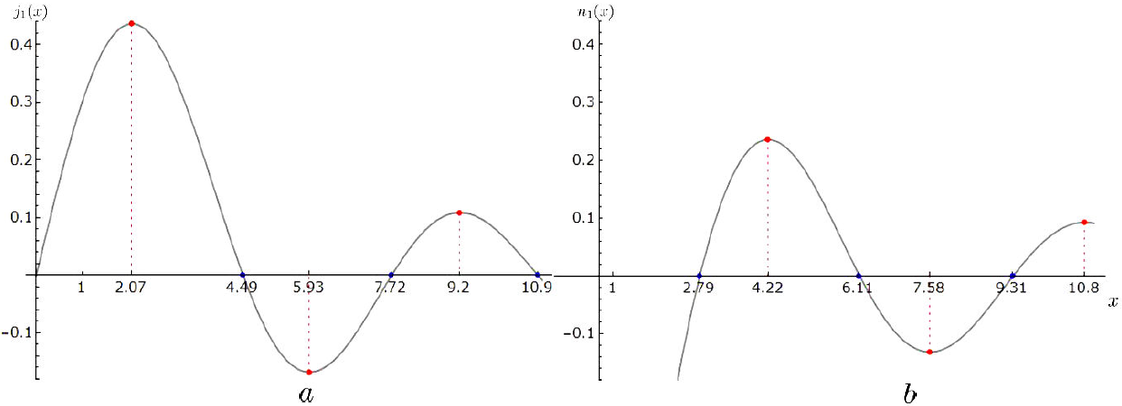
Figure 1. Plot of the real and imaginary parts of the spherical Hankel function:
j1(ka) and
n1(ka), respectively,
singularazing their lowest roots:
x1;s and
y1;s , identifying the
nodal lines, including the resonant cavity modes, and the positions of
their extreme values:
Figures 2a ,b,c illustrate magnetic induction field lines of Eqs. (10) and (11) in their forms of Eqs. (17) and (18), inside and outside the spherical surface in black, on any meridian plane at a given instant of time. The alternating lines in red and blue are closed, exhibiting their solenoidal character, and have opposite circulation directions; their separatrices in green dashed circles indicate the vanishing of the field there. Notice also the discontinuities of the field lines at the spherical surface where the current is distributed, Eq. (12).
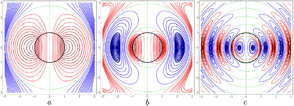
Figure 2. Magnetic induction field lines inside and outside the source spherical surface on black, in any meridian plane and at a given time, for the choices of (a) ka = 1, (b) ka = 2.0710 and (c) ka = 5.9280.
On the other hand, the conditions for the transverse electric TE modes of the
cavity with vanishing radial and polar components of the electric intensity can be
appreciated in Eq. (8), and the vanishing of the normal component of the magnetic
induction at the source boundary: j
1(ka) = 0 in Eq. (10) leads to the choices of the nodes
from Fig. 1. The appearance of this common
coefficient in the external electric intensity field, Eq. (9), and in the external
magnetic induction field, Eq. (11), leads to the vanishing of the electromagnetic
fields everywhere outside. Figures
3a, b, c illustrate the magnetic induction field lines in
the lower TE modes of the resonant cavity for the respective
frequencies:
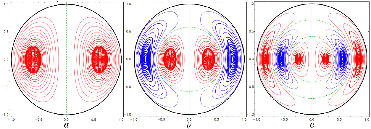
Figure 3. Magnetic induction field lines inside the spherical surface, in any meridian plane and at a given time, for the resonant TE cavity modes for (a) ka = 4.48724, (b) ka = 7.71886 and (c) ka = 10.9005.
It is relevant to emphasize that the field lines in Figs. 2 and 3 in the vicinity of the source spherical surface, both inside and outside, are dominated by the Faraday magnetoelectric and Maxwell electromagnetic inductions. Additionally, for the cavities the source distribution guarantees the vanishing of the fields outside.
It is very important to recognize that the results obtained so far are exact. Then, we analyze successively the quasi-static limit and the radiation limit. In fact, for the first one when
where the connection between the amplitudes A
0 and K
0 has been used from Eq. (14), and identifying the unit axial vector
The field outside, Eq. (11), takes the following form:
in which the angular distribution of an axial dipole moment and its inverse cube radial dependence are identified. The respective static magnetic dipole moments determining the fields inside and outside are
It is convenient to point out the different radial dependences of the coefficients in Eqs. (19) and (20): independent of the radius
On the other hand, in the far away zone where
then, the radial contribution to the field in Eq. (11) and the term in the derivative of r in the polar angle direction vanish sooner than the surviving term in the radiation zone:
Its companion electric intensity field from Eq. (9) becomes:
These are the exact results for the radiation fields from the sources distributed on the spherical surface, with a common amplitude determined by the value of j
1(ka) there, the same phase, perpendicular
3. Electric Dipole Sources and Fields
This section involves electric dipole distributions of surface charge density and linear current density along meridian half-circles on the spherical surface:
Both densities are connected by the continuity equation
which allows to obtain the relationship between their respective amplitudes:
and to convince the reader about their respective polar angle dependences.
Instead of constructing the scalar and vector potentials, we choose to construct the force fields from their inhomogeneous Helmholtz equation 11:
where
where its transverse source is the rotational of the current density, whose explicit form follows from Eq. (25):
For the dipole source of Eq. (32), only the term l = 1 in the sum of Eq. (30) is needed, thus
The unit vector in its cartesian components
projects into the
The first term vanishes because the Dirac delta function vanishes in both limits. Then the results inside and outside the source spherical surface become, respectively:
The magnetic induction field shows a discontinuity in its parallel circle components at the source spherical surface
according to Ampere’s law 11, measuring the magnitude of the meridian current distribution:
where the term inside the parenthesis is identified as ka times the negative of the Wronskian of the spherical Bessel functions: -i/k 2 a 2.
While the solution for the electric intensity field could be constructed from its sources, being the gradient of the charge density and the time derivative of the current distribution in Eq. (29), as we already did for the magnetic induction field, it is more expedient to use the Maxwell connection between both fields:
to obtain the electric intensity field as the rotational of the other one using Eqs.(36)-(37), with the results:
Notice the continuity of its tangential meridian components at the spherical boundary, as required by Faraday’s law. On the other hand, notice the discontinuity of its radial components at the same boundary in agreement with Gauss’ law:
leading to the same relationship of Eq. (27) for the amplitudes K
0 and
The electric field lines inside and outside the spherical boundary are defined by
which coincide with those of Eqs.(15)-(16). They have the same shape as those in Eqs. (17)-(18) but differ in their coefficients involving the derivatives of the product of the radial coordinate with the other Bessel function,
As in the previous section, the inclusion of the coefficient involving the other spherical Bessel function in each of these equations allows also the direct comparison of the field lines inside and outside the spherical surface: continuous in the contributions from the real parts, and discontinuous in the contributions from the imaginary parts associated with the Wronskian in Eq. (43).
Figures 5a,b,c illustrate the electric intensity field lines in the vicinity of the source spherical surface for increasing values of ka = 1, 4.48724, 7.71886, the last two corresponding to the nodes of Fig. 4a, which optimize the fields outside. The different colors of the lines inside and outside is due to the charge distribution on the spherical boundary, making their radial components discontinuous while their tangential components are continuous. In Fig. 5a the value of ka is too small and there are no nodal spheres inside. In Fig. 5b and 5c, one and two internal spherical nodes are recognized in green corresponding to extreme values in Fig. 4a. The lines outside have their respective spherical nodes determined by the nodes in Fig. 4b, alternating their directions in between. Notice the field lines leaving or arriving perpendicularly, from or to the source spherical surface, and becoming tangential to the first outer spherical node.
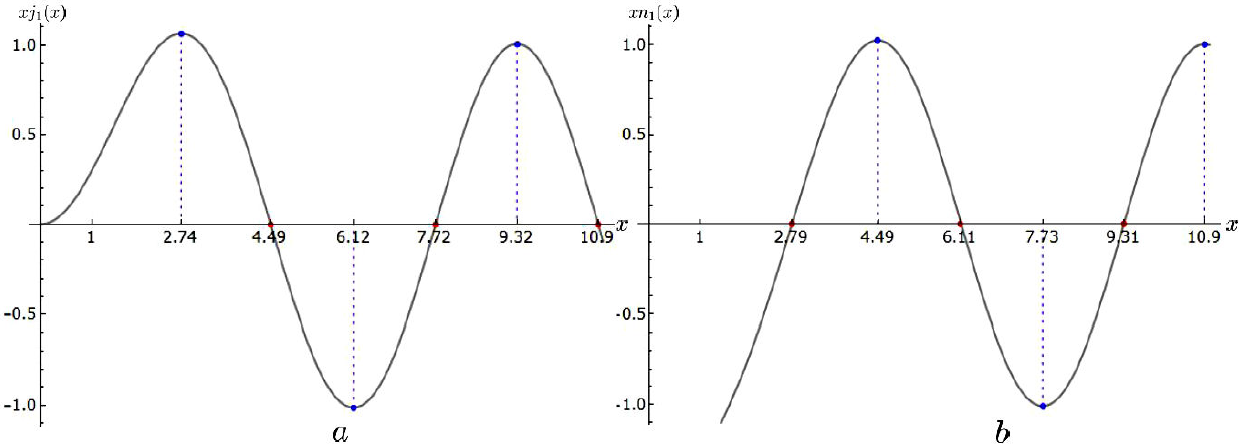
Figure 4. Plot of the real and imaginary parts of ka times the spherical Hankel function: (ka)j1 (ka) and (ka)n1(ka), respectively, singularazing their lowest roots, optimizing the radiation by antennas, and the positions of their extreme values identifying the inner nodal lines and the resonant cavity TM modes; the outer nodal lines are those of n1(ka), Eq. (47).
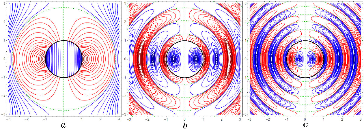
Figure 5. Electric intensity field lines inside and outside the source spherical surface on black, in any meridian plane and at a given time, for the choices of (a) ka = 1, (b) ka = 4.48724 and (c) ka = 7.71886.
On the other hand, the conditions for the transverse magnetic TM modes of the cavity with vanishing radial and polar components of the magnetic induction can be appreciated in Eq., and the vanishing of the tangential polar component of the electric intensity at the source boundary: (d/d(ka))[kaj 1(ka)]=0 leads to the choices of the extremes from Fig. 4a. The appearance of this common factor in Eqs. (37) and (42) leads to the vanishing of the electromagnetic fields everywhere outside. Figures 6a, b, c illustrate the corresponding field lines inside for the resonant TM cavity modes with respective frequencies: ω = (2.74371, 6.11676, 9.31662), in units of c/a, associated with the extreme values in Fig. 4a with 0, 1, and 2 nodes, respectively. They originate and end perpendicularly, from and to the source spherical surface, consistent with Gauss’s law. In Fig. 6a there are no internal nodes. In Fig. 6b and 6c the lines leaving or arriving from and to the spherical surface also become tangential to the neighbouring inner spherical node; moving farther in, the reader may identify the similarity with the field lines in Figs. 3a and 3b.
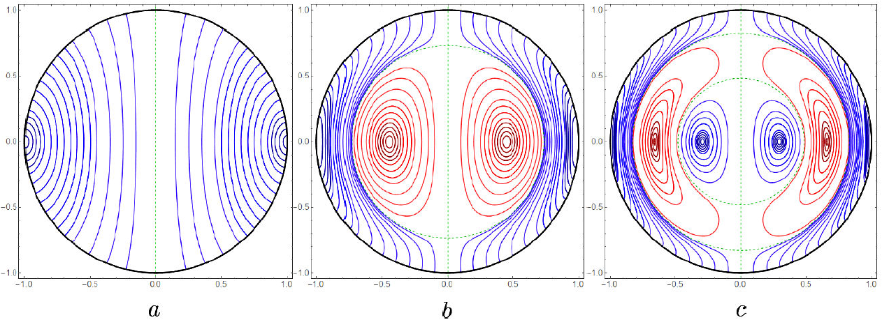
Figure 6. Electric intensity field lines inside the source spherical surface on black, in any meridian plane and at a given time, for the resonant TM cavity modes: (a) ka = 2.74371, (b) ka = 6.11676 and (c) ka = 9.31662.
We also analyse the quasi-static and radiation limits for the exact results obtained so far. For the first limit,
where the identification between the amplitudes K
0 and
The field outside Eq. takes the form:
in which the angular distribution of an axial electric dipole moment and its inverse cube radial dependence are identified. The different directions and space dependences of the field inside and outside, Eqs. (48)-(49), are accompanied also by the difference in their respective static electric dipole moments:
On the other hand, in the far away radiation zone where
and its companion magnetic induction field outside in this limit from Eq. (37) becomes:
These are exact results for the radiation fields, produced by electric dipole sources distributed on the spherical surface, sharing the same amplitude, the same phase, being perpendicular to each other, their vector product
4. Discussion
This section contains successively a summary and discussion of the quantitative and illustrative results in Secs. 2 and 3, a comparison of their similarities, differences and complementarities, as well as the formulation of some comments of didactic interest.
In the case of the magnetic dipole source, Eq. (1) describes its current parallel circle field lines and dipolarity on the boundary spherical surface. The corresponding vector potential, Eqs. (2)-(6), and electric intensity evaluated as the time derivative of the latter, Eqs. (7)-(9), share the direction and angular dipolarity of the source, as well as the radial dependence and the respective coefficients in terms of the spherical Bessel functions, ordinary and of Hankel type, inside and outside, respectively; both are continuous at the boundary spherical surface. The magnetic induction is evaluated as the rotational of the vector potential, Eqs. (10)-(11), inside and outside, with radial and polar components in each meridian plane; their radial components at the spherical boundary are continuous, consistent with Gauss’ law; while their polar components show a discontinuity at the same boundary, connected with the dipolar current source as required by Ampere’s law, Eqs. (12)-(13), leading to the relationship between the potential and source amplitudes, Eq. (14); the field lines inside and outside are also identified in their differential equation forms, Eqs. (15)-(16) and their integrated forms (17)-(18); they are the bases for Figs. 2a,b,c illustrating their behaviour in the vicinity, inside and outside, of the source spherical surface where the Faraday and Maxwell electromagnetic inductions come at play. Figures 3a, b, c correspond to the resonant cavity TE modes determined by the boundary condition of the vanishing of j 1(ka), which guarantees that the external fields also vanish, Eqs. (9) and (11).
On the other hand, the electric dipole source involves both a charge and a meridian half-circle current distributed on the spherical surface, Eqs. (42)-(25), connected via the continuity equation, Eq. (26), leading to the relationship between their respective amplitudes Eq. (27). The magnetic induction field satisfies the Helmholtz equation with the rotational of the current distribution as its source Eq. (28); it can be evaluated as the integral of the latter multiplied by the outgoing-wave Green function in its multipole expansion form Eq. (30). The rotational of the current distribution has parallel circle field lines with a sine of the polar angle dependence, as the original meridian current distribution; only the dipolar component in the mulipole expansion is selected by the angular integrations, Eqs. (33)-(34), and the magnetic induction field inherits the parallel circle field lines and the sine of the polar angle of its source; its radial dependence is that of the ordinary spherical Bessel and Hankel functions, inside and outside, with coefficients coming from the radial integration as the negative of the derivative of the product of the radial coordinate and the other Bessel function at the radius of the spherical boundary, Eqs. (35)-(37). The tangential components of the magnetic induction at the spherical boundary show a discontinuity, which by Ampere’s law Eq. (38) reproduces the original meridian current distribution, Eq. (39). The electric intensity is evaluated as the rotational of the magnetic induction via their Maxwell connection Eq. (40), with the explicit forms of Eqs. (41)-(42); exhibiting field lines in each meridian plane with a discontinuity in the radial direction at the spherical boundary connected with the surface charge distribution by Gauss’ law, Eq. (43), and consistent with the relationship between the charge and current amplitudes; the polar angle components are continuous, consistent with Faraday’s law; their field lines turn out to have the same shapes, Eqs. (44)-(45), as those of the magnetic induction for the magnetic dipole source Eqs. (15)-(16), allowing for the difference in their respective coefficients Eqs. (46)-(47) and Eqs. (17)-(18). Figures 5a, b, c illustrate their behaviour in the vicinity, inside and outside, of the source spherical surface, where the normal components are discontinuous, for increasing values of the frequency. Figures 6a, b, c illustrate the electric intensity field lines for the TM modes of the resonant cavities determined by the vanishing of the derivative of the product of the radial coordinate and the ordinary spherical Bessel function, or the positions of the extremes of such a product, Fig. 4a, guaranteeing also the vanishing of the external fields, Eqs. (37) and (42); notice that the field lines end radially at the source spherical surface where the charges are distributed.
From the comparative reading of the two previous paragraphs it is easy to recognize the similarities, differences and complementarities between the two types of magnetic and electric dipole sources and their electromagnetic fields. In the first one there is only the parallel circle dipole current distribution with the same properties inherited by the electric intensity; while in the second one there are both electric dipole charge and meridian current distributions. In the latter, the rotational of the current distribution exhibits parallel circle field lines and the same dipolarity; those properties are inherited by magnetic induction field with that rotational as its source. In turn, the magnetic induction in the first case has its field lines in meridian planes, continuous in their radial components at the spherical boundary, and discontinuous tangential components where the parallel circle currents are distributed; while in the second case the electric intensity has its field lines also in meridian planes, discontinuous in their radial components at the spherical surface boundary where the charges are distributed, and continuous in the tangential polar components. In the first case, the coefficients of the inner and outer spherical Bessel functions are the other spherical Bessel function at the spherical boundary, while in the second case the corresponding coefficients are the derivatives of the product of the radial variable and the other spherical function at the spherical boundary. These coefficients are the weight functions defining the respective dynamic dipole moments for the fields inside and outside. The vanishing of these coefficients also determine the corresponding frequencies for the respective TE and TM resonant modes of the cavities, making the outer fields vanish too.
Some of the following comments may help the reader understand the reasons for considering the sources to be harmonically distributed on a spherical boundary. This assumption allows us to recognize that inside and outside such a boundary there are no sources and, consequently, the electric intensity and magnetic induction fields are solenoidal; the rotational of one is related to the time derivative of the other one by Faraday’s and Maxwell’s laws; both are solutions of the Helmholtz equation. The harmonicity and the directions of the distributed sources are inherited by the respective fields. The problem of solving the Maxwell equations with well-behaved solutions inside and electromagnetic radiation solutions at very large distances, or no external fields outside a spherical cavity, subject to the conditions of satisfying Gauss’, Faraday’s and Ampere’s laws at the spherical boundary, is well defined. Here, we have illustrated their solutions for the magnetic and electric dipole cases. The solutions for higher multipoles can also be constructed.

