


 text new page (beta)
 English (pdf)
 Article in xml format
 Article references
 Send this article by e-mail
 Cited by SciELO
  Similars in
SciELO
Similars in
SciELO 
 Permalink
PACS: 01.40.Fk; 01.50.pa; 02.30.Nw
1. Introduction
The basic assumption of this work is to show how, in teaching and learning Mathematics and Physics, the close interrelation between the two disciplines and with Laboratory should not be circumvented or bypassed. On the contrary their interplay and mutual influence as well as their deep epistemological affinities should be promoted. In this framework Mathematics does not just provide tools for Physics but also drives physical insight; vice-versa Physics and its Laboratory can provide a simple access to Mathematical topics of not straighforward comprehension. Recent student learning investigations suggest that the understanding of Physics and Mathematics topics can be significantly facilitated by means of an integrated approach (see Fig. 1) with Laboratory activities, so allowing to enreach topics of meanings.

Figure 1. In undergraduate and graduate courses, Physics, Laboratory and Mathematics often tend to be autonomous through the delimitation of their frontiers and the building of specialistic languages. An open dialogue among Mathematics, Physics and Laboratory allows to confer to formal issues concrete form and utility and vice-versa allows to provide effective analysis tools to physical insights.
In other words, in undergraduate and graduate courses, disciplines as Physics and Mathematics are frequently set in an autonomous way by means of the delimitation of their frontiers, the building of specialistic languages and the employment of specific techniques and tools; such an approach furnishes points of strength to the single disciplines but at the same time furnishes the limits of the disciplinary knowledge. Disciplines are observation windows on the World, points of view on reality but if disciplines forget to be a part of a wider system of knowledge the interdisciplinary boundary limits become barriers and, in such a case, the word discipline recover its original meaning of whip for who intends to break the disciplinary walls.
In this reference contest, due to complexities encountered in dealing with time dependent frequencies, the study of variable length pendula as well as the study of Fourier and Wavelet transforms are rarely included within the program of Physics courses addressed to ungraduate and graduate students.
Such physical systems are characterized by a chirp-like time behavior, i.e. by local (i.e. time-dependent) pseudo-frequencies 1,2.
In the present work it will be shown how while Fourier Transform (FT) reveals an effective tool in analyzing stationary signals, in the presence of a time changing spectral content FT is not able to furnish detailed information on the different physical states of the oscillating system but provides only an average information on the motion frequency components; on the contrary in this latter case Wavelet Transform (WT) represents an effective tool for the time analysis of the non stationary signal allowing to precisely characterize the time variation of the oscillation motion frequency content 3,4,5. WT is nowadays extensively used in several fields of applications, such as audio, images, light and neutron scattering spectra analysis, spectroscopy, geophysics time series, biology and medicine 6,7,8,9,10,11,12,13,14,15,16.
In the following, in order to analyse the dynamics of a pendulum with a time-varying length, we apply both the FT with the WT approaches putting into evidence the pros et cons of the two analysis techniques.
2. Comparison between Fourier and wavelet transforms - historical background
From the historical point of view it is useful to mention that in 1822, Joseph Fourier, French mathematician and physicist who accompanied Napoleon on his Egyptian campaign, published the treatise titled “Theorie Analytique de la Chaleur” where he introduced the idea of expanding functions in sine or cosine trigonometric series to solve the heat conduction equation he had developed.
Starting from this study, FT allows to decompose a signal and to reconstruct it without loss of information even if such an analysis is localized in frequency but not in time; in other words FT allows to properly analyse stationary signals 17.
In order to overcome the limitations of FT a new analysis has been introduced later; such an analysis consists in introducing a “window” function of given length which slides along the time axis to execute a “time-localized” FT. This approach gives rise to the Short Time Fourier Transform (STFT) which was first introduced in 1946 by Dennis Gabor, a Hungarian mathematician. Gabor chose as window function a Gaussian but soon he realized that STFT furnished an equal resolution in time for lower and higher frequencies and that the width of the window function was the same for the entire analysis process 18.
In the mid 1970s Jean Morlet, a French geophysics working for an oil company, while investigating the acoustic echoes sent into the soil for identifying the existence of oil on the earth’s crest, developed the method of scaling and shifting the STFT. In order to analyse such echoes, Morlet first employed the STFT and observed that when holding constant the width of the window function the analysis didn’t run well; so, he proposed to maintain fixed the frequency of the window function and to change the width of the window by a dilatation or compression procedure 19.
This new approach led to the term “ondelette” introduced by Jean Morlet et Alex Grossmann in 1984. At first, the term was French and then was translated in English as wavelet:
i.e. wave (onde) and let (petite). Figure 2 shows the historical route of the wavelet concept genesis which starting from Joseph Fourier with FT (1822), through Dennis Gabor with STFT (1946), arrives to Jean Morlet (1984) with WT.

Figure 2. Historical route of the Wavelet genesis which starting from Joseph Fourier with FT (1822), through Dennis Gabor with FTFT (1946), arrives to Jean Morlet (1984) with WT.
From a mathematical point of view Fourier series allow to decompose a periodic function f (x) defined for
where a0, ak and bk are the Fourier coefficient, defined as:
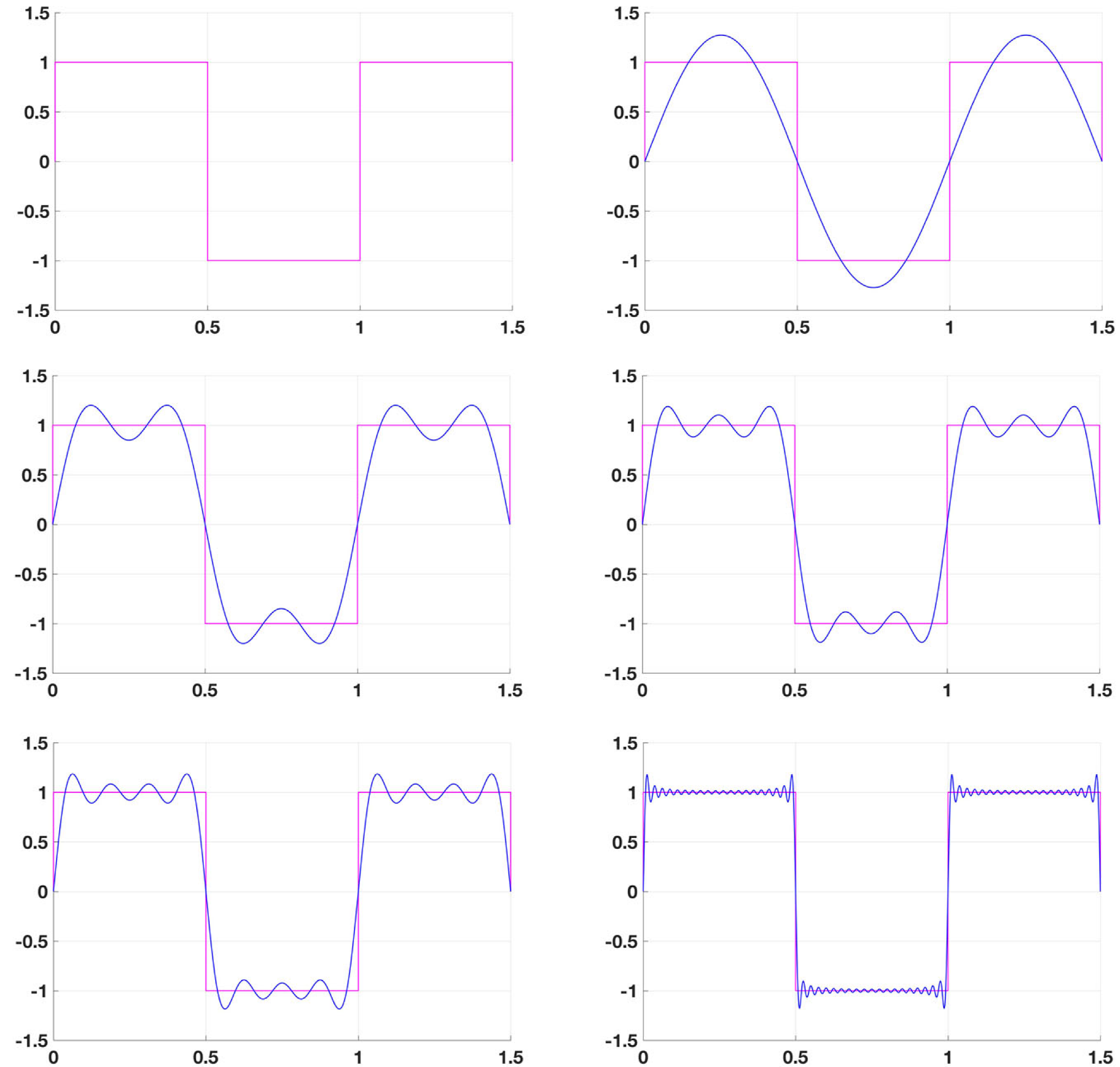
Figure 3 shows, as an example, the partial sums of the Fourier series for a square wave.
The Fourier Transform is an extension of the Fourier series to non-periodic functions which decompose it into a set of sine (or cosine) waves of different frequencies
It should be stressed that in such a case it is not possible to provide a connection between the frequency spectrum and the signal evolution in time.
On this regard, WT results more advantageous in respect to Fourier transform; in fact WT approach allows to decompose a signal into its wavelets components, by means of mother wavelet
where the parameter a > 0 denotes the scale and its value is the inverse of the frequency; the parameter
In Fig. 4, as an example, scaled and shifted versions of the mother wavelet are reported.

Differently from FT, which shows only which signal frequencies are present, WT, in addition, also shows where, or at what scale they are. Furthermore, while FT allows to decompose the signal only in cosine and sine component functions, the WT takes into account several wavelet mother functions, that can be chosen according to the similarity degree of the mother functions with the investigated signal 23,24,25,26,27,28,29,30.
In this paper, according to the behavior of the investigated oscillator, the wavelet Morlet has been chosen as mother wavelet:
where
It should be noticed that in the special case in which the wavelet mother is
3. Theoretical background
Let us first focus the attention on a pendulum, a toy physics system full of lots of meanings (see Fig. 5), of length

From the physical point of view the dynamics of such a system can be obtained by applying the fundamental second law equation dynamics equation:
where a is the acceleration, F is the total force acting on the mass,
Being:
it results:
and
Under the hypothesis that the pendulum length during the oscillation changes with a constant rate, i.e.
Under these assumption, Eq. (10) becomes:
and making the further assumption that
whose solution can be put under the form:
where:
4. The experimental setup and results
The experimental set-up includes:
a spherical mass whose weight is 100 g;
a fixed support to fix the pendulum;
a step by step rotating device for changing the pendulum length;
a computer equipped with data acquisition program (Logger Lite) and spreadsheet (Excel);
an ultrasonic sensor device to measure the distance between itself and the oscillating mass which directly transmit the recorded data to a PC.
As far as the experiment procedure is concerned, the pendulum motion was sampled through a GoMotion-Vernier sensor. The system length variation as a function of time was assured by the step by step rotating device and was registered through a PC.
During the first part of the experience, the condition in which the pendulum length is fixed was investigated, reiteratly registering the motion at different pendulum lengths. The oscillation period evaluated for different lengths is reported in Fig. 6 that, as expected, fulfills the expected
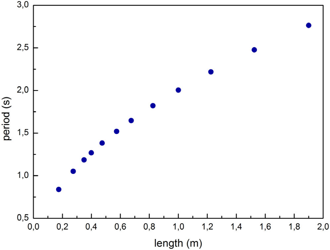
Figure 6. Behavior of the oscillation period T as a function of the pendulum length under stationary conditions.
First, we have studied the system under stationary conditions, i.e. at fixed pendulum length, and then we have investigated and the analyzed, by a WT approach, a set of measurements in which the length changed linearly as a function of time 42,43,44,45,39,40. In Fig. 7, as an example, the length variation versus time plot is reported. As it can be seen the pendulum length as a function of time fulfils a linear trend with a constant slope of

Figure 7. Length variation versus time. The pendulum length as a function of time fulfils an linear trend with a slope of -0.025 m/s.
Figure 8 reports a picture of the analyzed signal. In particular, on the top, the collected oscillation signal in the condition of length change is shown. It is clear that oscillation frequency increases with time. FT, that is reported on the right of the picture, provides only an average of the frequencies of the investigated signal; while, on the bottom of the picture, the WT scalogram shows that the oscillation pseudo-frequency changes with the time.

Figure 8. Comparison of the investigated signal analyzed by means of FT and WT. More precisely, on the top of the figure the collected oscillation signal, under the condition of varying length is shown; on the right of the figure its FT showing only an average of the registered signal frequencies; on the bottom of the figure the WT scalogram that shows how the oscillation pseudo-frequency changes with time.
5. Conclusion
The present paper shows an example of how it is possible to promote a fruitful alliance among different disciplines on a specific study case which allows to access in an user-friendly way to mathematical operations such as Fourier and Wavelet transforms. Both these approaches have been applied to characterize the effects of the pendulum length change on the following time-dependent oscillation frequency. It is shown that WT outperforms the FT approach highlighting which frequencies are present (as FT) and, in addition, where they are, so providing an easy-to-interpret physical significance of time-frequency analysis.

