


 text new page (beta)
 English (pdf)
 Article in xml format
 Article references
 Send this article by e-mail
 Cited by SciELO
  Similars in
SciELO
Similars in
SciELO 
 Permalink
PACS: 07.79.Lh; 62.20.de; 68.35.Gy
1. Introduction
Nanotechnology is a topical issue of scientific rigor about studying phenomena and manipulation of materials at its smallest scale. Its applications and areas of development make it an essential subject in the curriculum of any undergraduate engineering student. However, applying these concepts into practice in a laboratory can be difficult because of the required instrumentation. This paper presents a laboratory practice on the characterization of materials by atomic force microscopy (AFM). The main objective is to get, in a quantitative manner, the modulus of elasticity of different samples by analyzing the experimental force-distance curves acquired in an AFM working in contact mode.
Being that the AFM is a characterization technique of surface materials, it’s a suitable technique in a vast area of applications such as synthesis, friction, wear, and functionality of diverse surface modified materials. During the development of this practice, students are expected to show evidence which reflects the concepts studied and to present the information in a professional and consistent style. Meanwhile, students will be able to improve their presentation and writing skills related to the themes of research and analysis of the current literature, Hertz’s contact mechanics, Computational statistics, and data analysis.
The present paper intendeds to specify the theoretical background of AFM force plots as well as to present a selection of measurements that can be implemented with this apparatus. The next section is a general introduction to AFM contact mode including: working principle, the technique employed for the calibration of the instruments, and the fundamentals of the theory concerning the force-distance curves. The analytic procedure to obtain the substrate stiffness is stated in detail. After an overview of calibration problems and model limitations, the main experiments concerning the measurements of the Young’s Modulus are exposed, pointing out the main established results.
2. Theoretical Framework
AFM was first introduced in 1986 by Binning, Quate and Gerber. The universal character of the repulsive forces between the tip and the sample, which are employed for surface analysis in AFM, enables the examination of a practically unlimited range of materials 1. AFM has developed into a multifunctional technique suitable for characterization of topography, adhesion, mechanical, and other properties on scales from hundreds of microns to nanometers 2-4.
Results gathered from the piezoelectric sensor in the AFM is crucial for characterizing materials in the Nano and Pico scale. A force-distance curve is obtained by monitoring the vertical displacement of the cantilever (δc or deflection) with respect to the piezoelectric actuator height (Zp) 5. The tip-sample force can be expressed in terms of Hooke’s law:
For characterizing the spring constant of the cantilever (kc) the thermal tune method was used by analyzing the power spectral density of the cantilevers free oscillation affected due to thermal noise. If the microlever is modeled as a harmonic oscillator, the equipartition theorem implies that in thermal equilibrium the oscillator has an average energy related via the mean square deflection
This method is used owing its geometry and composition independency. However, two corrections should be considered for an improvement. The first, a factor relating that we can’t measure all the oscillation modes (sometimes only the first mode or Z1) of the cantilever in the
Unfortunately, the distance controlled by the AFM’s control loop (Zp) is not the real tip-sample distance (S or separation) but the original distance between sample surface and the cantilever. These are different because of cantilever deflection (δc) and sample deformation (δs or indentation) 9 but are linked in a way that:
Since the only distance that one can control is the piezo-displacement, after the F−Zp plot is acquired an axis change can be made (F − Zp + δc) so that the indentation values (that will be used for further analysis) can be visible as negative values from a F −S curve (real force-distance curve) as stated by Eq. 4 and presented in Fig. 1.
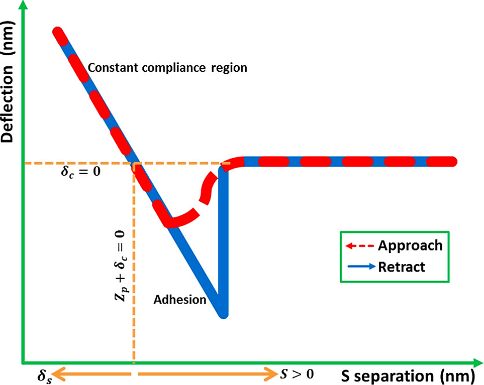
Figure 1 Schematic of a typical deflection-vs.-separation plot (δc − vs − S), with S = δc + Zp. Indention depth appears as negative values of S. The abscissae axis is not at scale.
The AFM tip is able to probe a very small interaction area. With this, the tip gives it a high sensitivity to very small forces 10. This will let us work in the elastic regimen of our materials. In this type of experiment (contact between a rigid sphere and a flat surface) Hertz contacts mechanics 11 states that for the case of a nonrigid spherical indenter and sample, the distance of mutual approach (δ') between two distant points within the indenter and the sample is given by:
where R is the relative curvature of the indenter and the sample, E the elastic modulus of the sample and k is an elastic mismatch factor 12 given by:
In Eq. 6, Es vs and Et, v t are the Young’s Modulus and Poisson ratio for the sample and the indenter respectively. When the indenter is perfectly rigid, k = 9(1− v)/16, and the distance of mutual approach δ' is the penetration depth δs below the original sample 12.
Following Johnson insights, 13 it can be stated as an effective or equivalent elastic modulus of the system (ETOT) Eq. 7, so that Eq. 5 can be written in function of this value.
where F is the load applied and R can be approximate as the indenter radius for small indentations. It can be noted that the effective elastic modulus of the system decreases as the indenter becomes less rigid. Therefore, the distance of mutual approach δ' for a nonrigid indenter is greater than that for a rigid indenter due to its deformation 12. Fortunately, that kind of displacement is recorded by the AFM’s photodetector so that from the data recorded indentation values can be obtained.
Although AFM has a great potential for characterization of surface properties, it is important to realize that contact mode force spectroscopy is a technique with some limitations and difficulties, being AFM nanoindentation a better approach 14,15. One of the most crucial aspects is cantilever calibration. Indeed, to withstand the force exerted by the probe, the microlever’s sensitivity (deflection vs. voltage ratio) should be well known; calibration with an infinitely hard surface that could leave us to pure cantilever deflection (and zero sample deformation) is required. The harder the calibrating surface the more accurate the sensibility, though the damage of the tip apex is increased.
A second source of problem is related to the size and shape of the AFM probe. The tip’s radius of curvature is an important variable in our calculations, and manufacture parameters are not that precise. Therefore, characterization of the cantilever’s probe should be realized (e.g. electron microscopy) at the beginning, taking into account that it won’t be a constant parameter due to the flattening of the tip that may occur in the course of the experiments.
Ultimately, an important limitation is the contact model used. Several theories define the elastic deformation of the sample, and their differences arise due to the adhesion in the tip-sample system. In the Hertz model, the adhesion of the sample is neglected, whereas other theories take account of it outside (Derjaguin-Müller-Toporov) or inside (Johnson-Kendall-Roberts) the contact area. Butt and Capella 8 stated that in these last theories, the work of adhesion W can be calculated from the jump-off-contact, if the tip radius R is known. Then it is possible to calculate δ as a function of the effective elastic modulus ETOT. The JKR model is used in the case of large tips and soft samples with a large adhesion, while the DMT model is used for small tips and stiff samples with a small adhesion 8. Notwithstanding, all of these models are only approximations.
3. Materials and Methods
All samples were observed in an open environment on a Multimode NanoScope IIIa (Veeco Metrology Group) coupled with a Signal Access Module (SAM). Data were exported to text files using the microscope’s software package. All force values were calculated using non-conductive silicon nitride (Si3N4) triangular cantilevers (Veeco model NPS-10/NP-20) with a length of 120/205 μm and nominal spring constant from 0.5 to 0.06 N/m depending on which of the 5 types of cantilevers were used (different for each alumni team). Due to our didactic approach, samples with easily differentiated values are necessary so that, even with our theoretical assumptions, measurement errors and students’ misinterpretations can converge to one of the possible samples, which are High Density Polyethylene (HDPE), Highly Ordered Pyrolytic Graphite (HOPG ZYH), Laminate (glass) GFRP, Glass D263M, Gold, Copper UNS C11000, Stainless Steel type 304, and Tungsten Carbide/Cobalt 94/06.
In order to get the spring constant of the cantilever, the appropriate connections between the SAM and the Microscope had to be made first, using a BNC cable so the data of the photosensor sensibility can be obtained (“In 0 Output” to the “Aux B Input”) Then the cantilever, which was to be calibrated, was placed in the microscope and engaged on a hard surface, after configuring it in contact mode.
After this, the first force curve in units of Volts is acquired. Because deflection in units of distance is required instead of voltage, the cantilever’s sensitivity needs to be attained from this force curve, using the marker tools on the monitor. Next, to achieve thermal oscillation data, a scan of 0.1 nm, 512 lines, and 61 Hz of the “Aux B channel” are required. The raw data, which represents the thermal noise oscillations, are exported as a vector to a text file for further analysis.
To capture the force-distance curves for the given samples, the microscope in contact mode is used. Entering the values of sensibility and spring constant, force values can be acquired. Once the force curves were transformed into indentation curves by Eq. 4, the Young’s Modulus of the materials analyzed can be calculated through the Hertz model (Eq. 8). Different values for the elastic constant are retrieved from one curve so that a Gaussian fitting of the results is expected 16.
4. Results and Discussion
After importing the thermal oscillation data into MATLAB, we obtained a vector of length 262144 (which is 512 * 512, the amount of readings taken with the microscope). It is important to remember that the time interval (∆t) between each one of these values is 16.01 µs (corresponding to the reciprocal of 61 Hz*512*2); because of this, a new vector “t” with 262144 values of time starting at 0, and increasing in intervals of 16.01 µs, is created. The plotted deflection against time vectors are presented in Fig. 2a and consists of thermal noise from which quantitative data can’t be obtained directly.
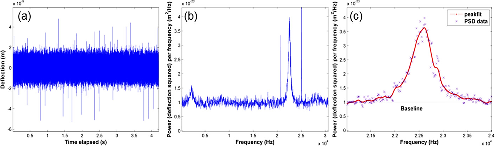
Figure 2 Three different steps in the process of measuring the cantilever spring constant. (a) Typical thermal noise plot obtained from the raw data of thermal oscillation measured with the microscope. (b) PSD analysis of (a). (c) Close-up of the resonant peak, with a smoothing fit.
In order to analyze the data, it is necessary to transform the values from the time domain to the frequency domain, performing a power spectral density (PSD) analysis.
Said analysis can be easily performed using the MATLAB function “pwelch”, which calculates an estimate of a function’s PSD using Welch’s method for spectral estimation using modified periodogram; 17 the function receives as an input: the thermal noise data vector, the sampling frequency of 62462 Hz, N=4096 data point segments, a window length equal to N for the Hamming window, and a default overlap value of 50 %.
Two new vectors are then obtained from the previous routine: a frequency vector (Hz) and a PSD vector (m2/Hz). After plotting said vectors, a graph like the one in Fig. 2b is obtained where it can be seen that a specific frequency dissipates most of the energy.
The next step is to get the area under that resonant peak, for which MATLAB’s curve fit toolbox proves useful. After loading the desired data with the “data” feature, the “fitting” feature must be used to apply an appropriate smooth fit to the peak data (as shown in Fig. 2c); and finally an integration can be performed with the “analysis” feature to obtain the value of the area under the resonant peak (subtracting the area below the “baseline” of average thermal noise) that represents
If the peak area was obtained in units of m2, then the constant will be in units of N/m as expected; different cantilevers’ spring constant values were obtained with this method. The comparison with their nominal values are condensed in Table I:
Table I Nominal and experimental values for the cantilever spring constant of different cantilevers.
| Cantilever type |
Nominal Kc (N/m) |
Obtained Kc (N/m) |
Relative error |
| NPS10-C | 0.24 | 0.2018 | 15.9 % |
| NPS10-B | 0.12 | 0.1144 | 4.6 % |
| NP20-B | 0.12 | 0.1146 | 4.5 % |
| NP20-A | 0.58 | 0.3684 | 36.4 % |
| NPS10-A | 0.35 | 0.3377 | 3.6 % |
It must be noted that the nominal values for spring constants are subject to much variation; they are given by the company as an expected value for the general manufacturing process (and specific tips may deviate too much from that value); also, the spring constant may be altered by frequent use of the cantilever.
The data obtained from the samples with the AFM’s force mode were again exported to .txt files so they can be read by MATLAB, which we’ll use to perform the numerical analysis. The exported values consist of a four column vector, each measuring 512 in length. Two for the approaching curve and two for the retracting curve. To compute elasticity, the analysis should be done with the approaching curve. One column corresponds only to the values of δc in nm. The other relates the separation values (Zp + δc), also in nanometers. Multiplying the latter by the spring constant of the cantilever previously calculated, force values can be obtained.
When plotted, these values produce a graph, such as the one presented in the dotted line of Fig. 1. Interpreting the graph, and reading it from right to left, the tip of the cantilever approaches the sample with very little variation on the force; when the tip is just about to make contact, the force drops slightly because of the attractive Van der Waals interaction, but it soon rises because of the short-range Coulomb repulsion forces that come into play. Then the force reaches a stable value and stays there on the left side of the graph. Another important aspect to notice in this graph is the point where the tip of the cantilever is already in contact with the sample and is being deflected upward.
This point can be detected either visually (“data cursor” tools ) or by calculating the differences between the loading and unloading curves, using peak find instructions and changes in sign of the first and second derivate.
The contact point is translated to the origin in order to obtain a loading-indentation curve like the one presented in Fig. 3c. When multiplied by the spring constant of the cantilever, the Y axis corresponds to the applied load F, for which there is a specific indentation δ. These are the values that are to be plugged in the Hertz model (Eq. 8) to get the effective elastic modulus (ETOT) of the samples. Once obtained, the Young’s Modulus of the sample (Es) can be calculated with Eq. (7).
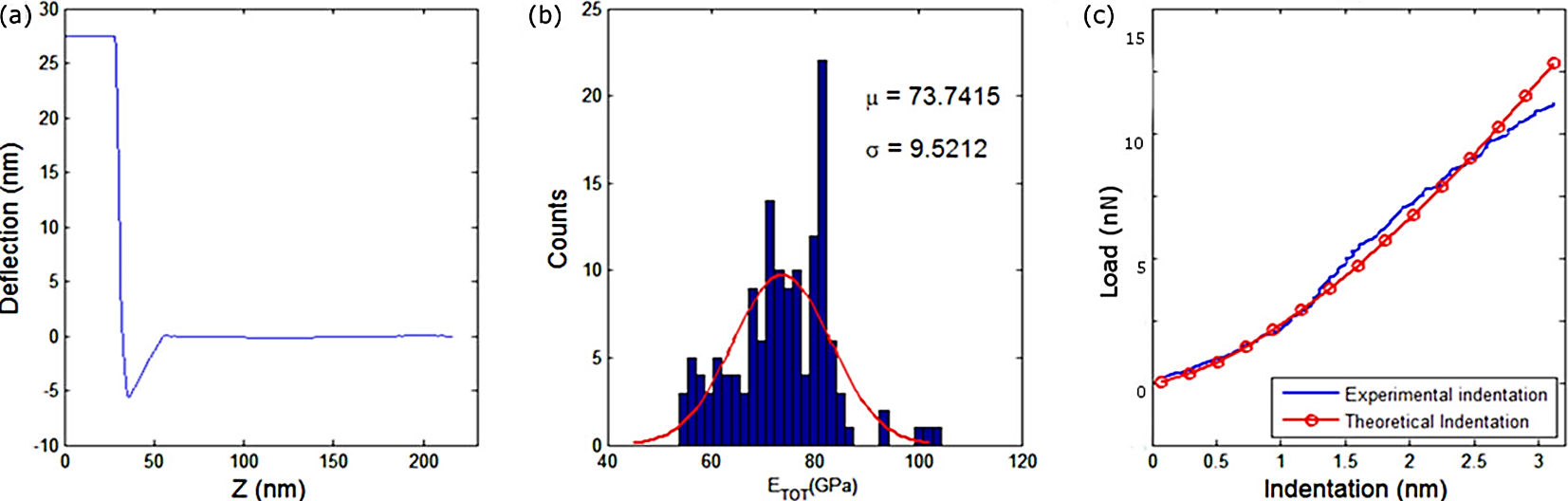
Figure 3 Elastic properties of materials. (A) A typical force curve for a gold substrate. (B) Histogram of the effective elastic modulus computed for the approach curve in (A). (C) Contrast of the theoretical indentation (segmented line) and the experimental indentation curve.
However, several effective elasticity moduli can be obtained for each material with this method. Thus, the data points are presented in a histogram (Fig. 3b). A Gaussian Fitting is implemented to visualize the mean and distribution of each modulus, for every material. These results are presented in Table II. Values of Young’s Modulus and Poisson ratio for theoretical values can be found elsewhere 18, for Si3N4 cantilevers, the values used where 290 GPa and 0.3 respectively 19.
Table II Mean values of the effective elastic modulus (ETOT) compared to the theoretical values of ETOT. Relative error is presented for each material analyzed.
| Material | Theoretical ETOT [GPa] |
Experimental ETOT [GPa] |
Relative error |
| HDPE | 0.96 | 1.3±0.4 | 35.4 % |
| HOPG ZYH | 19.5 | 16.9±4.7 | 13.7 % |
| GFRP | 25.5 | 21.9±6.3 | 14.1 % |
| Glass D263M | 59.4 | 47.7±7.1 | 19.8 % |
| Gold | 69.9 | 73.7±9.5 | 5.3 % |
| UNS C11000 | 89.2 | 75.4±9.3 | 15.5 % |
| SS304 | 123.6 | 99.2±14.9 | 19.8 % |
| Tungsten Carbide/Cobalt |
177.6 | 128.4±23.4 | 27.7 % |
5. Conclusions
We have presented an analysis and interpretation of force-distance curves in order to obtain the elastic modulus of different materials. For quantitative data analysis, the spring constant of the cantilever was obtained also practically with the thermal tune method achieving great accuracy. The contact mode in AFM was used for data acquisition and, although some model limitations, the procedure can be considered as effective for the most part as the values obtained are related to the expected values. These discrepancies are attributed to tip geometry and adhesion forces. Further analysis can derive from the calculation of Hamaker constants from the distance of interaction of the pull-down force in the approach curves due Van der Waals body-body interaction.
Being that the AFM is an affordable characterization technique for any engineering laboratory, its implementation as a teaching tool is simple and productive. The final product of this practice is a report including all the subjects discussed in this paper. At the implementation in the classroom, students failed to identify the scope and limitations of the theory and experimentation. Also, a large number of incorrect citations and an improper theoretical framework were present, showing the students’ poor ability to understand concepts and transform knowledge from them. This field was the most emphasized in later works, showing improvement. However, this work fulfills its purpose of introducing undergraduate students not only to the concepts of nanotechnology but also to the concepts of experimental analysis, which made this a rewarding experience.

