3.1. Nuclear Spin

The particles that make up the atomic nuclei (protons and neutrons) have the intrinsic quantum mechanical property of spin. In nuclear physics the total angular momentum that the nucleus has is called nuclear spin ¹⁸, though the term should not be confused with spin of each nucleon or total spin as the sum of all nucleons, because this is just one of the two contributions to the nuclear spin, the other is the angular momentum of the nucleons. So each nucleon will have a net angular momentum such that:

then the nuclear spin will be:

or just:

Each of these vectors have a similar quantum number. The magnitude of orbital angular momentum satisfies:

The direction of the angular momentum vector L is associated with the quantum number m. For a given quantum orbital momentum number l, there are 2l +1 integral magnetic quantum numbers m ranging from −l to l. Along the z axis the component of angular momentum is given as:

For the vector of spin angular momentum S, its quantum number s can take integer or half-integer values:

and for the z component, we find that s_z = m_sℏ, there are 2s + 1 values of m_s. To exhibit the property of MRI, the nucleus must have a non-zero value of s. In medical applications, the proton (₁H) is the nucleus of most interest, due to its high natural abundance, however other nuclei have been studied.

The proton is a fermion whose value of s is 1/2, therefore there will be two possible values for S_z, i.e. ±ℏ/2. The eigenfunctions describing the nucleus can be written as |+1/2〉 and |−1/2〉, and since in quantum mechanics every physical observable has an associated operator, we can write an eigenvalue equation to describe the observation of the spin state as:

where S_z is the operator describing the measurement of angular momentum along the z axis.

3.2. Voxel magnetization

To measure the energy of the spin system it is necessary to construct a Hamiltonian operator. The shape of the Hamiltonian can be derived from classical electromagnetism, for the energy of a magnetic moment placed in a magnetic field ¹⁵. The nuclei have a magnetic moment μ⃗ which is proportional to the spin angular momentum ⁴:

where γ is a constant of proportionality called gyromagnetic ratio, which for the proton it has a value of 2.675×10⁸ rad/s·T. When this magnetic moment is placed in a magnetic field B its ground state is degenerated and the energy of a particular level will be:

combining Eqs. (6), (7) the Hamiltonian is obtained:

and since the field B is oriented in the z direction, the Hamiltonian becomes:

now using Schrödinger’s equation, the energy eigenstates are found

and they will be:

For the proton m_s = ±1/2, a transition between the two states represents a change in energy. This is called Zeeman splitting¹⁷ and is shown in Fig. 1, where it shows that as the intensity of the magnetic field increases, the energy difference between the states is bigger. The two possible states are more commonly known as “spin−up” and “spin−down”, where the latter has a higher energy state than the “spin−up” state. Transitions between the two states can be induced by absorption or emission of a photon such that:

Figure 1 Energy level diagram for a Zeeman interaction. 

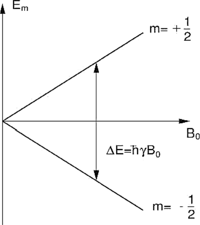
Thus obtaining the Larmor equation which underpins the whole phenomenon of Nuclear Magnetic Resonance.

The characteristic frequency ω₀ is called Larmor frequency and B₀ = B_z. In a real system there is not only an isolated nucleus, but many nuclei which may occupy a particular spin state. This means that our development must be extended to consider an ensemble of spins. To do this we define a Ψ eigenstate, which is a linear combination of possible spin states for a single nucleus as:

When performing a measurement on the system, the expected value of the operation on this superposition of states is:

where the value |a_ms|² represents the probability of finding a single nucleus in the m_s state. For the case of a proton, which is the particle of interest, with two spin states we have:

The ratio of the population in the two energy states follows the Boltzmann statistics ⁴,

and since k_BT ≫ ℏγB₀, expanding the first order exponential we have

and the difference in the number of spins between the spin-up state and the spin-down state will be:

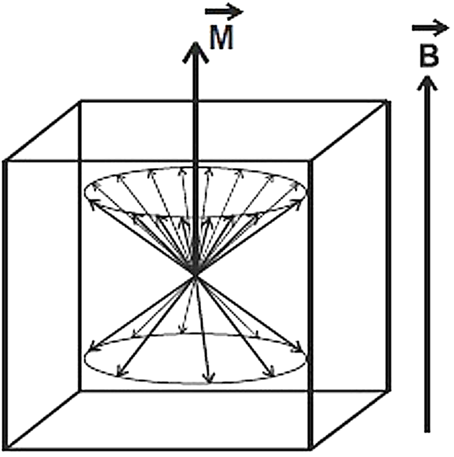
The magnitude of the magnetization of a voxel containing a nucleus density ρ is obtained by multiplying the density by the difference between the number of spins in both states and the magnetic moment of the nuclei µ_z = ±(γℏ/2)

The magnetization of the volume element also has a direction which is equal to the orientation of the main magnetic field for that reason it should be considered as a vector quantity, as it shown in Fig. 2.

Figure 2 Magnetization vector of the volume element ⁶. 

3.3. Excitation of the Magnetization by radio-frequency pulse

A volume element of the sample is defined as a voxel. Having placed a transmitting antenna in the direction of maximum emission to the voxel in the vertical plane and changing the transmission frequency, when we emit the frequency of precession (Larmor frequency), the nuclei are able to absorb energy, i.e. enter resonance.

When the nuclei of the voxel are entering into resonance, the magnetization vector M travels performing a spiral rotational movement relative to the direction of the field B ₀. Each nucleus entering into resonance at a specific frequency specified by the Larmor Law, depending on B ₀ perceived and biochemical environment in which it is located. Therefore, the radio-frequency emission contains an approximate bandwidth of 100 kHz.

Separation of M with respect to its equilibrium position is determined by the angle of inclination or FLIP angle. Its value depends on the power and time of radio-frequency emission, among other factors.

The process of the radio-frequency emission is of the order of microseconds called radio-frequency pulse and quantified by the value α. A 90° pulse moves the magnetization vector about the xy plane, and a 180° pulse inverts the magnetization respect to its equilibrium position.

After a 90° pulse, the longitudinal component of the magnetization vector is zero, in this position the number of nuclei in the lower energy state equals the number of nuclei in the higher energy state, it is called a state of saturation.

3.4. MRI selectivity

If we have multiple voxels placed under different magnetic fields, we can selectively excite either by simply changing the transmission frequency of the antenna.

A magnetic gradient enables atomic nuclei to perceive a distinct magnetic field. In addition to changes in biochemical environment, one can selectively resonate all nuclei within positions that are being excited by the frequency bandwidth used in the pulse emitter. Therefore all voxels contained in a plane perpendicular to the direction of the gradient plane and whose thickness depends, once defined the value of the gradient, on the bandwidth used on the pulse emitter, will be excited.

Magnetic resonance images are obtained by sending pulses to different spaced time intervals with suitable values, which is a pulse sequence.

3.5. Evolution of magnetization under temporal variation of the magnetic field

Taking a volume element (Voxel) that has a magnetization vector M, the set of equations describing the temporal evolution of said vector are called Bloch equations¹ and are defined as follows:

where γ is the gyromagnetic ratio of the proton and M₀ = M is the magnitude of the magnetization in equilibrium, T₁ and T₂ are time constants that will be discussed later. The above equations can be solved with the appropriate conditions; for example, immediately after when the radio-frequency pulse is turned off:

3.6. Nuclear relaxation

Once the radio emission is completed, the magnetization vector, M, returns to its initial position by releasing energy through a process called relaxation. Relaxation occurs because nuclei emit the excess energy absorbed when entering resonance. Relaxation ends when the proportion of nuclei voxel between higher energy states and lower energy states match the Boltzmann equilibrium.

The return to the equilibrium position of M produces magnetic field modifications that may be collected by a receiving antenna, since the magnetic field variations induce an electrical signal called Free Induction Decay (FID) ¹⁶, which is a damped sinusoidal signal. The frequency of the sinusoid is the precession frequency imposed by the value of the magnetic field during relaxation.

Given the definition for the electromotive force (fem) and the magnetic flux through a coil:

On the other hand, for the magnetization vector M of a sample, there is an associated magnetic field from the current

density

the vector potential derived from a source is defined as:

with this, the magnetic field can be calculated as B=▽⃗×A, and we can write the flux through the coil as:

Substituting the vector potential in the term for the current density and later in the line integral, we have:

simplifying the above equation and performing integration by parts:

The expression in the parentheses of Eq. (60) can be compared with the vector potential A, obtaining an expression for circuits:

thus the curl of the line integral is indeed the magnetic field per unit current that would be produced by the coil at point r'

The magnetic flux through the coil can be written as:

Finally, the electromotive force is expressed as:

Two voxels placed under different magnetic fields in the moment of relaxation, will have different relaxation frequencies and, therefore, their signals may be differentiated through a frequency analysis such as Fourier analysis. By studying signals of relaxation, one can obtain information on the density (D) of hydrogen nuclei in the voxel and information related with the medium by the parameters T1, T2, and T2 *.

3.7. Spin-lattice relaxation (T1 relaxation)

During the relaxation, the hydrogen nuclei release their excess energy. Once reaching complete relaxation, the magnetization vector M recovers its initial value aligned with the direction of the main magnetic field B₀. An analysis after a pulse of radio-frequency of the variations in time of the projection of the magnetization vector on the longitudinal axis (M_z), called longitudinal relaxation, once the value of the projection is identical to the initial value of M, the relaxation will be over. Thus the study of the longitudinal relaxation gives an idea of the rapidity with which it again reaches its initial state.

As we can see in the Fig. 3, the longitudinal relaxation has the form of a growing exponential regulated by a time constant expressed in milliseconds called T1, which is also called Longitudinal Relaxation Time.

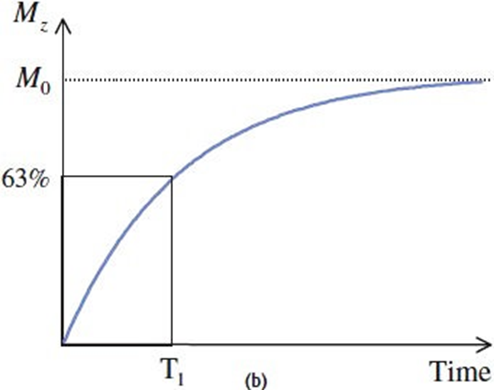
Figure 3 The recovery of M_z to M₀ is controlled by an exponential. T1 is the necessary time to recover the 63% of the equilibrium value of the magnetization ⁴. 

The values of T1 increases with the value of the magnetic field.

3.8. Spin-spin relaxation (T2 Relaxation)

We can get information related to the biochemical structure of the medium, by studying the variations over time of the component for the magnetization vector in the vertical plane (x,y) during the transverse relaxation.

When M_x,y is zero it implies that the magnetization vector is aligned on the z-axis with the main magnetic field. Immediately after excitation, part of the spins precess synchronously, these spins have a 0° phase and are said to be in phase, this state is called coherent phase.

The coherent phase is gradually lost as the spins advance and others are delayed on their way precession. In other words the transverse relaxation is the decay of transverse magnetization due to loss of coherence in the spins.

The transverse relaxation differs from longitudinal ralaxation in that the spins do not dissipate energy to the surroundings but, rather, exchange energy with each other.

The evolution of the transverse magnetization over time, until it vanishes, corresponds to a sinusoid with a dampened relaxation frequency generating an exponential decay (see Fig. 4). This exponential decay of the surroundings is regulated by a parameter T2* ². When we take into consideration all factors that influence the asynchronism of the nuclei, or T2 if neither are influenced by the external magnetic field’s inhomogeneities or local magnetic variations acting permanently on the nuclei. Therefore T2 indicates asynchronism of nuclei of the voxel during relaxation due to spin-spin random influences which depend on the composition and structure of the tissue. T2 is the time that must elapse before the transverse magnetization loses 63% of its value. The time constant T2 is called the Transverse Relaxation Time.

Figure 4 T1 and T2 simultaneously happen, but T2 is much faster than T1 ⁴. 

Returning to the coherence, it is lost in two ways: