


 nueva página del texto (beta)
 Inglés (pdf)
 Artículo en XML
 Referencias del artículo
 Enviar artículo por email
 Citado por SciELO
  Similares en
SciELO
Similares en
SciELO 
 Permalink
PACS: 42.25.Gy; 42.25.Lc.
1. Introduction
The movement of a spinning top has always raised the curiosity of experts and non-experts; basically, it is due to the stability that the spinning top acquires while rotate. Although the explanation of its behavior is not immediate in mechanical terms, from Euler and Lagrange is understood the dynamics of this movement, and its theoretical aspects are found in books of advanced mechanics 1-3.
Despite of the extensive literature one can find regarding to theories about the spinning top and the gyroscope 4-7, there are very few reports about the measurements of precession and nutation rates. In pioneering works, by using stroboscopes, people could measure: angular velocity, inclination angle and the path of the spinning top tip over coal or graphite paper; but they did not provide velocities of nutation and precession 8.
Currently, by using high speed video cams, those measurements can be directly done. This kind of methodology is used on projects or experiments for university labs, however, in this case collecting numerical data is a difficult task because it requires a shot reproduction, frame by frame, in order to determine the body’s trajectory as a function of time 9.
In this work, we present a simple way to find, for a certain time interval, the measurements for velocities of: precession, nutation, and rotation, in a gyroscope; all this by using a single picture and a laser light adhered to the gyroscope, which is projected over a horizontal plane. To compare experimental values with theoretical, we use an approximate solution for Euler equations for the problem of symmetrical spinning top with fixed point by using Riemann stereographic projection on the horizontal plane.
2. Gyroscope Movement
Generally, a gyroscope is a rigid body with axial symmetry that can rotate around a fixed point on its symmetry axis. In particular, it consists of a rod with a fixed point on its middle and which has the freedom of self-orienting in any direction inside a specific angular range. At the same time, the rod has a rotating disk located on one of its ends whose axis coincides with the rod. At the other end, the rod also has a counterweight which allows adjusting the center of mass for the system.
The most notorious thing of this instrument is the fact that when the disk rotates speedily, the center of mass does not fall to the lowest position, instead, it keeps moving slowly in a horizontal circle with fast nodding motion in the axis of rotation.
The movement in a gyroscope is composed by three independent movements: 1) Rotation, which is the disk movement on its own axis; 2) Precession, which is the average horizontal movement done by the disk axis around a vertical, and 3) Nutation which corresponds to small and fast oscillations of the axis. Usually, Nutation has small amplitude and tends to quickly disappear under friction; this is why frequently it goes unnoticed.
2.1. Movement equations of a gyroscope
On the basis of an inertial system, the rate of change of components from angular
By aligning the base vectors from the rotating system with the main axes of a gyroscope, the
Momentum of Inertia Tensor becomes diagonal, I =
diag(I1; I2;
I3),, and components from the angular moment
will depend only on the respective components of angular velocity,
Li =
Iiωi . Now, by aligning
Gyroscope’s orientation is fully described by three Eulerian angles corresponding to the angles that relate the main axis of a gyroscope with the coordinate axis on a steady state system

The total angular velocity is a vector addition of angular velocities associated to each one of Euler’s angles. Figure 1 shows that the angular velocity components based on a rotating system are:
On the other hand, the torque exerted by gravitational force with respect to the fixed point, is given by a vector product between the center of mass position
where μ ≡ mgh is the maximum torque. In the case where this torque was the only contribution to torsion momentum of system (neglecting friction), then the products of
Although approximately, the direct solution of Euler’s equations gives an intuitive method to correctly describe the movement of a gyroscope. To find out such a solution, is advisable to work in the complex plane, so that we add the first equation from (2), to the second one which was previously multiplied by the imaginary number i; all this to obtain the following complex equation:
with τ ≡ τ1 + iτ2 and ω ≡ ω1 + iω2. From (3) and (4) is obtained for these complex quantities that τ = μ sin θe-iψ and ω = Ωe-iψ , where Ω ≡ (̇θ + i̇ϕ sin θ).By using these values on (5), and factorizing the exponential e-iψ , the following expression appears:
This is a differential equation on the real variables θ and ϕ, and can be expressed in terms of complex variable as
This variable corresponds to Riemann’s stereographic projection of a point on the sphere in the plane 13; here, the real part is directed to

By differentiating the expression (7) respect of time, we obtain
and
Replacing (8) and (9) on Eq. (6) the following equation shows up:
here, according with (7), cosθ = (1-|a|2)/(1+|a|2). Equation (100), together with ̇L3 = τ3 are equivalent to Euler’s equations (2). This equation is a generalization to θ large for the gyroscope’s equation used in external ballistic 14.
2.2. Approximate Solution to the gyroscope’s equation
Equation (10) is not linear, of second order on the complex variable a, and is not analytic. The exact solution for this equation is not easy to find. However, an approximate solution for small nutation can be easily obtained. In this case the value of θ can be replaced, on first approximation, by the mean value θ0. After changing variables
Eq. (10) can be rewritten as:
The roots of the right hand polinomy on (12) are given by
which corresponds to the fast precession frequencies s+ and slow s-15. The differential Eq. (12) can be solved by separating variables followed by an integration using partial fractions, thus obtaining
where x = βt cosθ0 + c, being c a complex constant of integration. The imaginary part of c is the relevant quantity because the real part may be eliminated through a temporal translation. Having on mind the definition of s given in (11), the value for a is obtained after integrate and exponentiate (14)
where A' is a constant resulting from the integration. The function sin x is proportional to
with A and B arbitrary constants. On the limit when B → 0 a slow precession solution for a is given, the case when B → ∞ (with AB finite) leads to a fast precession solution. Generally, precession turns out to be of lower frequency than nutation, therefore the solution for nutation of small amplitude corresponds to (16) with |B| ≪ 1. By making a binomial approximation of the term inside parenthesis in (16), we have
where ωn and ωp are frequencies of nutation and precession respectively, given by
Expression (17) implies that a is the sum of two rotating vectors of constant amplitude, |ap | and |an |, which spin with frequencies ωp and ωp + ωn respectively. Because of the fact that the amplitude of precession movement is greater than that of nutation, and its frequency is lower, the trajectory that vector a presents in a plane has a shape of rosette. On expression (18) ωn is defined positive, and from (19) can be seen that ωp has the same sign as μ. The rosette shape formed on the projection plane comes given by the relative sign between frequencies of precession and nutation, which means depends on the sign of μ. When the frequencies have the same sign (μ > 0) the projection created on the plane has the apices pointing inward, while if signs are opposite (μ < 0), the apices on the projection are going outward (See Fig. 3).

Figure 3 Graphic representation of the gyroscope solution, (a) for μ > 0 and (b) for μ < 0. ϕn y ϕp are the arguments of an and ap , respectively.
The precession frequency does not diverge for θ
0 approaching = π/2, despite first appearances. In this limit is
obtained ωp
= μ/L
3, like the simple theoretical expression for precession frequency
found in most elementary physics textbooks, and ωn
= L
3/I
1. They also correspond to the expressions of frequency values on the
limit of fast rotation
From Eqs. (19) and (18), can be found relations between precession and nutation frequencies which are independent of the state of movement, given by:
Given that
This relation predicts that the number of rotations by nutation tends to the value I1/I3 for θ = π/2 or L3 large, but in general (23) has a linear behavior with respect to the parameter (ωp /ωn )cosθ0, where the slope and the axis intersection are determined by I1/I3.
Finally, to obtain the expressions of these angles as a function of time, solution (17) and definition (7) are equating, and considering |an /ap | ≪ 1 we got:
and except a constant
where δ is the argument of an /ap . From this last expression is evident that the mean value of the angular velocity ϕ is the precession velocity ωp , while for tanθ/2 is |ap |, what we make to coincide with tanθ0/2, having an relative uncertainty of order (|ap |/|an |)2.
Results aforementioned coincide with the Lagrangian description in the approximation of harmonic potential to first order in the parameter
3. Experimental section
3.1. Experimental Assembly
With an experimental set up we looked for a corroboration of the gyroscope solution, Eq. (17), with its corresponding parameter values, fits in an exactly way to an experimental situation. For this experience was used a Pasco ME8960 gyroscope, it consist of a disk of 1.755 ± 0.001 kg mass with a radius of 12.7 ± 0.1 cm and a thickness of 2.0 ± 0.1 cm, which can spin around an axis with little friction, at the same time this axis may be orientated in any azimuthal direction but inside a range of 30° to 140° respect to the zenith. The orientable axis has a fixed point at 12.7 ± 0.1 cm from the disk, which is pivoted at 30.7 ± 0.1 cm from the floor over a vertical bar. This bar is nailed in the center of an A-shaped base of molten iron, and it can rotates around its own axis. At the opposite end of orientable axis, opposite to the disk, there is a counterweight that works to vary the position of the center of mass.
To visualize the a vector, a simple laser pointer device is set up in such a way that it remains on the same vertical plane than orientable axis, but presenting an angle with respect to the vertical equal to half of zenithal angle of the axis. This can be achieved by setting the pointer on the base of an isosceles triangle where one of its congruent sides aligns with the vertical bar and the other with the orientable axis, as showed in Fig. 4.

To have information about the angular velocity of rotation from the disk, an electric switch was installed to the pointer device so, it turns on during half of revolution cycle and then turns off on the other half. The switch was fixed by sticking a copper semi-disk to one of the faces of the spinning disk. The laser’s feeder circuit becomes closed only when two small brushes, in contact with the disk, also get in touch with the cooper semi-disk, thus the circuit is open every half revolution. (see Fig. 4).
In our case the laser light is projected upward over a horizontal screen 70 cm away from floor, which is formed by a framed fabric in a way that the luminous dot can be observed over the screen. A mirror just above the screen works as a guide of images from screen to the digital camera; the camera is installed in a tripod, on side of the mirror and pointing out to it, as can be seen in Fig. 5.

By taking a photography of luminous dot in a time interval large enough is obtained a discontinuous light beam, each segment of the bright line along with the following dark interval, correspond to a disk rotation. Initially counterweights were set on the disk axis in a way that the center of mass will stay just on the pivoted point from orientable axis. Later, an additional counterweight, with a mass of 151.48 ± 0.01 g, was set on one of the orientable axis ends. Experiments with the counterweight on the same disk side at 21.0 ± 0.1 cm from pivoted point (forward) were made, and then with the counterweight on opposite side (backward) to 34.5 ± 0.1 since pivoted point. The counterweight mass value multiplied by the pivoted point distance and by the constant of gravity, accounts for the maximum torque μ to which the gyroscope is subjected. Given the laser pointer position, with an additional counterweight ahead, the rosette shape formed by the movement of the dot of light shows its apices outward; reciprocally, by adding the counterweight back, rosette’s apices point inward, as show Fig. 3.
3.2. Results
With the mass values of both, counterweights and disk, and taking into account their position, the calculation of values for the main inertia momentum and maximum torque, related to each situation of additional counterweight, is direct. These values are given by Table I.
Table I Values for inertia moment and maximum torque in both positions of additional counterweight.
| I1(g·m2) | I3(g·m2) | μ(g·m2/s2) | |
| Counterweight forward | 100 ± 1 | 13.3 ± 0.1 | 316 ± 1 |
| Counterweight backward | 112 ± 1 | 13.3 ± 0.1 | 512 ± 1 |
The disk was set up to spin around the orientable axis at a specific velocity ψ and certain value of θ0. The system was left to evolve and the trajectory of luminous dot was photographed, with a digital camera which has an aperture time control, inside a dark room. The camera was located above screen and by over the gyroscope, an exposure time of 10 seconds for each photo was set, also a green laser was used which is why the result of each photography is a dotted green line with a dark background. After inverting colors using an editor of images, pictures are seen as a red trace with white background.
From photographic records is obtained: an angular interval of a nutation Δϕ, the number of rotations per nutation Δn, the total number of rotations n, and the circumference diameters D1 and D2, intern and extern, tangent to the trajectory of luminous dot. The values of these diameters must be given using units of a reference diameter Dr, which is defined as the trajectory diameter of luminous dot when gyroscope precesses uniformly with θ = π/2. These measurements, along with the exposition time t, allow us to find the frequencies of rotation, precession and nutation, as well as the average value of zenithal angle, through next relations:
Using these values, and according to (21) and (22), relations given by μ/I1 and I1/I3 can be calculated. 60 pictures of each counterweight, back and front, were analyzed. Figure 6 shows one example of each case, where the way how every measurement was obtained is described. The average values of these quantities are called experimental values; the associated uncertainty is the standard deviation of data, divided by square root of the amount of data. Theoretical data correspond to those obtained from Table I. The average values for μ/I1 and I1/I3, experimental and theoretical, are shown in Table II.

Figure 6 Pictures of the projection of gyroscope movement with inverted colors. Counterweight ahead and back respectively.
Table II Theoretical and experimental values for μ/I1 and I1/I3.
| Forward | Backward | |||
| μI1(s-2) | I1I3 | μI1(s-2) | I1I3 | |
| Theoretical | 3.16 ± 0.03 | 7.51 ± 0.07 | 4.57 ± 0.04 | 8.47 ± 0.08 |
| Experimental | 3.20 ± 0.03 | 7.42 ± 0.02 | 4.58 ± 0.02 | 8.53 ± 0.02 |
According to (23) the graphs of ωn in function of (ωp cosθ + ωn )-1, present a linear form with a slope of μ/I1.
Figure 7 shows the experimental results using counterweight back and then ahead. Solid lines represent theoretical values.

Figure 7 Experimental value of μ/I1 for experiments with counterweight ahead (light circles), and with it on back (dark circles).
A kind of dispersion in values can be noticed; it possibly is because of a high value of the relative uncertainties on Δn. If it is only considered one nutation cycle, it shall an uncertainty of order 1/Δn, which, in our case is around 12%. In order to diminish the uncertainty, N cycles of nutation are taken, reducing the error in one factor of 1/N. However, for low velocities, N cannot be too large because the Δn variation per cycle of nutation will be significantly affected by friction, therefore on the beginning exists an insuperable limit on precision of measurements, determined by the disk friction.
Figure 8 shows experimental results for the number of rotation per nutation as a function of the relation between precession and nutation frequencies, multiplied by cosine of θ0. Solid lines represent theoretical values.

Figure 8 Relation between the number of revolutions per nutation cycle for the experiments with the counterweight ahead (light circles) and back (dark circles).
Figure 9 shows the ratio between experimental precession speed ωp
and the expected in the simplest model μ/L3, as a function of the parameter
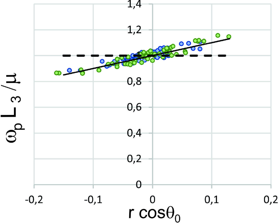
Figure 9 Relationship between experimental precession speed !p and its expected value μ/L3 in the simplest model, in function on the parameter
For the data reported in Fig. 7, 8 and 9 the rotation frecuency was between 3 to 13 revolutions per second.
4. Summary
By using Riemann projections, Euler’s equations for a symmetric spinning top with a fixed point are solved, in an approximate way, when considering nutations of small amplitude. Under this approximation, the solution corresponds to the addition of two rotating vectors on the complex plane, and their velocities of rotation will define both velocities of precession and nutation for a spinning top.
The Riemann projection was visualized through an intermittent light of a laser. A photographic register of luminous dot projection allowed us to obtain in an easy and simple way, quantitative information of rotation, precession and nutation velocities, and the zenithal average angle of gyroscope; which may be expensive and complicated using different methods.
From the photographic record of laser dot trajectory on a horizontal plane, the parameters of movement for a total of 120 experiments were determined. Theoretical expressions are verified experimentally.
From the parameters obtained by photographic records, quantities μ/I1 and I3/I1 were found, and then were compared with the direct measurement of these on the mass distribution of gyroscope. Although there was some dispersion, the average on measurements is adjusted in a precise way with theoretical data.
Experimentally was shown that the number of rotations per nutation cycle is a lineal function of the relation between velocities of precession and nutation, and the average inclination angle of gyroscope axis. The slope and intercept with the axis coincide, inside the range of uncertainty, with the values predicted by the model.
The analysis made on this work does not considered the friction due to air viscosity, although the photographic registers evidence this effect; this is an indicator of the high level of sensibility in this experiment. Nevertheless, because relatively small intervals of time were taken, these effects were ignored.

